This work is licensed under a Creative Commons Attribution-ShareAlike 4.0 International License

About this document¶

This document was created using Weave.jl. The code is available in on github. The same document generates both static webpages and associated jupyter notebooks jupyter notebook.

$$\def\indep{\perp\!\!\!\perp} \def\Er{\mathrm{E}} \def\R{\mathbb{R}} \def\En{{\mathbb{E}_n}} \def\Pr{\mathrm{P}} \newcommand{\norm}[1]{\left\Vert {#1} \right\Vert} \newcommand{\abs}[1]{\left\vert {#1} \right\vert} \DeclareMathOperator*{\argmax}{arg\,max} \DeclareMathOperator*{\argmin}{arg\,min} \def\inprob{\,{\buildrel p \over \rightarrow}\,} \def\indist{\,{\buildrel d \over \rightarrow}\,}$$

Introduction¶

The bootstrap is a method of inference that utilizes resampling. The basic idea is as follows. Suppose you have some parameter of interest for which you want to do inference. Let $T_n$ denote some test statistic involving the estimator. The test statistic is a function of data, so the distribution of the estimator is a function of the distribution of data. Let $F_0$ denote the exact, finite sample distribution of the data. Let $$G_n(\tau, F_0) = \Pr(\hat{\theta}_n \leq \tau)$$ denote the exact finite sample distribution of the statistic. To do inference, we would like to know $G_n(\tau, F_0)$. This is generally impossible without strong assumptions. Asymptotics get around this problem by approximating $G_n(\tau, F_0)$ with its asymptotic distribution, $G_\infty(\tau,F_0)$. The bootstrap is an alternative approach (but the formal justification for the bootstrap still relies on asymptotics). The bootstrap approximates $G_n(\tau, F_0)$ by replacing $F_0$ with an estimate, $\hat{F}_n$. One common estimate of $\hat{F}_n$ is simply the empirical CDF. When observations are independent, we can randomly draw $T^\ast_n$ from $G_n(\tau, \hat{F}_n)$ by randomly drawing with replacement a sample of size $n$ from the orgininal observations, and then computing $T^\ast_n$ for this sample. We can do this repeatedly, and use the distribution of the resulting $\hat{\theta}^\ast_n$’s to calculate $G_n(\tau,\hat{F}_n)$.

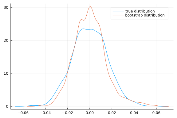
As a quick example, here’s some code where the statistic is the sample median minus its true value.

using Plots, StatsPlots, Distributions, Optim, ForwardDiff, LinearAlgebra, GMMInference
Plots.gr();

dgp(n) = rand(n)
estimator(x) = median(x)
# simulating T ~ G_n(τ,F_0)
n = 1000
S = 999
T = [estimator(dgp(n)) for s in 1:S] .- 0.5
function bootstrap(data, estimator, S)
  n = length(data)
  θhat = estimator(data)
  T = [estimator(sample(data,n, replace=true)) for s in 1:S] .- θhat 
end
Tboot = bootstrap(dgp(n),estimator, S)
density(T, label="true distribution")
density!(Tboot, label="bootstrap distribution")

References¶

Mackinnon (2006)¹ and MacKinnon (2009)² are good practical introductions to the bootstrap. Horowitz (2001)³ is also a good overview, and includes more precise statements of theoretical results, but does not contain proofs. The lecture notes of Shi (2012)⁴ are another very good overview. Gine (1997)⁵ is a rigorous and fairly self-contained theoretical treatment of the bootstrap.

Although the bootstrap works in many situations, it does not always work. For example, Abadie and Imbens (2008)⁶ show the failure of the bootstrap for matching estimators. See Andrews (2000)⁷, Andrews and Han (2009)⁸, and Romano and Shaikh (2012)⁹ for theoretical developments on situations where the bootstrap fails and alternatives that work. Hall (1994)¹⁰ gives a theoretical overview of when the bootstrap provides asymptotic refinement. Chernozhukov, Chetverikov, and Kato (2017)¹¹ discusses the bootstrap in high dimensional models.

Theory¶

This section follows the approach Van der Vaart (2000)¹². We focus on the case where $T_n = \frac{\hat{\theta}_n - \theta_0}{\hat{\sigma}_n}$ is a t-statistic. A simple and useful result is that if $T_n$ and $T^\ast_n$ both converge to the same distribution, then the bootstrap is consistent.

Proof sketch: $T_n$ and $T_n^\ast$ both $\leadsto T$ immediately implies $$G_n(\tau, F_0) \inprob G_\infty(\tau)$$ and $$G_n(\tau,\hat{F}_n) \inprob G_\infty(\tau),,$$ where $G_\infty(\tau)$ is the CDF of $T$ . This implies that $$G^{-1}_n(\tau,\hat{F}_n) \inprob G^{-1}_\infty(\tau)$$ for all $\tau$ where $G_\infty$ is continuous. Then we have $$\Pr(\theta_0 \geq \hat{\theta}_n - G_n^{-1}(\tau, \hat{F}_n) \hat{\sigma}_n) = \Pr\left(\frac{\theta_0 - \hat{\theta}_n}{\hat{\sigma}_n} \leq G_n^{-1}(\tau, \hat{F}_n)\right) \to \Pr(T \leq G^{-1}_\infty(\tau)) = \tau.$$

This theorem is very simple, but it is useful because it suggest a simple path to showing the consistency of the bootstrap: simply show that $T_n^\ast$ has the same asymptotic distribution as $T_n$. Here is a simple result for when $T_n^\ast$ is constructed by sampling with replacement from the empirical distribution. We will let $\mathbb{P}_n$ denote the empirical distribution, and $x_i^\ast$ denote draws of $x_i$ from it.

Proof sketch it is straightforward to show that $\Er[x_i^\ast | \mathbb{P}_n] = \bar{x}_n$ and $Var(x_i^\ast|\mathbb{P}_n) = \bar{x^2}_n - \bar{x}_n^2 \to \sigma^2$. Applying the Lindeberg CLT then gives the result.

Pivotal statistics¶

The above results imply that the bootstrap works for both $S_n = \sqrt{n}(\bar{x}_n - \mu_0)$ and “studentized” a statistic $T_n = \sqrt{n}(\bar{x}_n - \mu_0)/\hat{\sigma}_n$. There is some advantage to using the later. A statistic is called pivotal if its distribution is completely known. If we assume $x_i \sim N$, then $T_n$ is pivotal and has a t-distribution. If we aren’t willing to assume normality, then the distribution of $T_n$ is unknown, but its asymptotic distribution is completely known, $N(0,1)$. Such a statistic is called asymptotically pivotal. $S_n$ is not asymptotically pivotal because its asymptotic distribution depends on the unknown variance. It is possible to show that the bootstrap distribution of asymptotically pivotal statistics converge faster than either the usual asymptotic approximation or the bootstrap distribution of non-pivotal statistics. See Hall (1994)¹⁰ for details.

Here is a simulation to illustrate.

dgp(n) = rand(Exponential(),n)
estimator(x) = mean(x)
θ0 = 1.0
N = [5 10 20 100]
B = 999
function simulatetests(n)
  function bootstrap(data, stat, S)
    n = length(data)
    T = [stat(sample(data,n)) for s in 1:S]
  end
  data = dgp(n)
  t = sqrt(n)*(mean(data)-θ0)/std(data)
  [cdf(Normal(),t),
   mean(t.<bootstrap(data, d->(sqrt(n)*(mean(d) - mean(data))/std(d)), B)),
   mean((mean(data)-θ0) .< bootstrap(data, d->(mean(d)-mean(data)), B))]
end
res=[hcat([simulatetests.(n) for s in 1:1000]...) for n in N]

p = 0:0.01:1
global fig = plot(layout=4, legend=:none)
for i=1:4
  plot!(fig,p, p->(mean(res[i][1,:].<p)-p), title="N=$(N[i])",
        label="asymptotic", subplot=i)

  plot!(fig,p, p->(mean(res[i][2,:].<p)-p), title="N=$(N[i])",
        label="pivotal bootstrap", subplot=i)
  plot!(fig,p, p->(mean(res[i][3,:].<p)-p), title="N=$(N[i])",
        label="non-pivotal boostrap", subplot=i)
end
fig

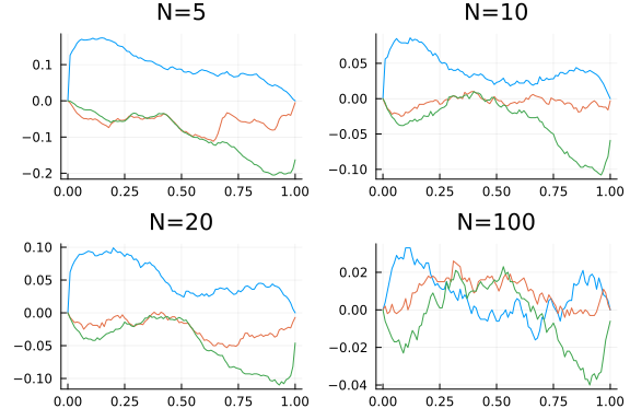
This figure shows the simulated CDF of p-values minus p. For a perfectly sized test, the line would be identically 0. The blue lines are for the usual t-test. Green is from bootstrapping the non-pivotal statistic $\sqrt{n}(\bar{x}^\ast - \bar{x})$. Red is from bootstrapping a pivotal t-statistic. As expected, the red line is closer to 0, illustrating the advantage of bootstrapping a pivotal statistic.

Bootstrap does not always work¶

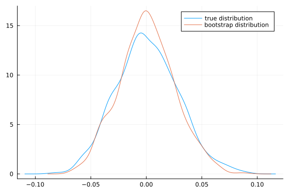
It is important to remember that the bootstrap is not guaranteed to work. A classic example is estimating the mean squared. Let $x_i \sim F_0$, where$F_0$ is any distribution with mean $\mu$ and variance $\sigma^2$. The parameter of interest is $\theta = \mu^2$. The estimator will be $\hat{\theta} = \bar{x}^2$. The delta method and CLT imply $$\sqrt{n}(\bar{x}^2 - \mu^2) \indist 2\mu N(0,\sigma^2)$$ similarly conditional on the data, $$ \sqrt{n}(\bar{x^\ast}^2 - \bar{x}^2) \indist 2 \mu N(0,\sigma^2)$ $$ A problem occurs when $\mu=0$. The limiting distributions become point masses at 0. The CDF is no longer continuous, so the theorem above does not apply.

Here’s an illustration

function bootmeansquared(μ0, n)
  dgp(n) = rand(n) .- 0.5 .+ μ0
  estimator(x) = mean(x)^2  
  S = 1000
  T = [estimator(dgp(n)) for s in 1:S] .- μ0^2
  function bootstrap(data, estimator, S)
    n = length(data)
    θhat = estimator(data)
    [estimator(sample(data,n,replace=true)) for s in 1:S] .- θhat 
  end
  Tboot = bootstrap(dgp(n),estimator, S)
  density(T, label="true distribution")
  density!(Tboot, label="bootstrap distribution")
end
bootmeansquared(0.5,100)

bootmeansquared(0.0,500)

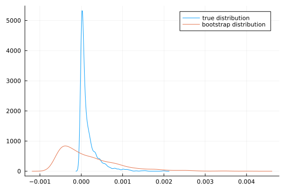
Depending on the random numbers drawn (in particular, whether the simulated sample mean is very close to 0 or not), the above picture may look okay or terrible for the bootstrap. Try running it a few times to get a sense of how bad it might be.

Bootstrap for GMM¶

Joint hypotheses¶

The failure of the bootstrap for the mean squared when the true mean is 0 has important implications for GMM. In particular, the AR statistic,

$$AR(\theta) = n [1/n \sum g_i(\theta)]' \widehat{Var}(g_i(\theta))^{-1} [1/n \sum g_i(\theta)]$$

is essentially a mean squared. If we naively attempt to apply the bootstrap by computing

$$AR(\theta)^\ast = n [1/n \sum g_i^\ast(\theta)]' \widehat{Var}(g_i^\ast(\theta))^{-1} [1/n \sum g_i^\ast(\theta)]$$

we will get incorrect inference. The problem is that we want to test $H_0: \Er[g_i(\theta)] = 0$, but in the bootstrap sample,

$$\Er[g^\ast(\theta)|data] = 1/n \sum g_i(\theta) \neq 0.$$

For the bootstrap to work, we must ensure that the null hypothesis is true in the bootstrap sample, we can do this by taking

$$AR(\theta)^\ast = n [1/n \sum g_i^\ast(\theta) - \bar{g}_n(\theta)]' \widehat{Var}(g_i^\ast(\theta))^{-1} [1/n \sum g_i^\ast(\theta) - \bar{g}_n(\theta)]$$

where $\bar{g}_n(\theta) = 1/n \sum g_i(\theta)$.

Here is a simulation to illustrate. It uses the same IV-logit share example as in the extremum estimation notes.

n = 100
k = 2
iv = 3
β0 = ones(k)
π0 = vcat(I,ones(iv-k,k))
ρ = 0.5
data = IVLogitShare(n,β0,π0,ρ)

function arstat(gi)
  n = size(gi)[1]
  gn = mean(gi,dims=1) 
  W = pinv(cov(gi))
  n*( gn*W*gn')[1]
end

function ar(θ,gi)
  n,m = size(gi(θ))
  1.0-cdf(Chisq(m), arstat(gi(θ)))
end

function bootstrapAR(θ,gi)
  giθ = gi(θ)
  gn = mean(giθ,dims=1)
  n = size(giθ)[1]
  S = 999
  T =hcat([ [arstat(giθ[sample(1:n,n,replace=true),:]),
             arstat(giθ[sample(1:n,n,replace=true),:].-gn)
             ] for s in 1:S]...)'
  t = arstat(giθ)
  [1-cdf(Chisq(length(gn)),t)  mean(T.>=t, dims=1)]
end

function simulatetests()
  data = IVLogitShare(n,β0,π0,ρ)
  bsp=bootstrapAR(β0, get_gi(data))
end

simulatetests (generic function with 2 methods)

pvals = vcat([simulatetests() for s in 1:500]...)
p = 0:0.01:1.0
plot(p, p->(mean(pvals[:,1].<p)-p),  label="asymptotic", legend=:bottomleft)
plot!(p, p->(mean(pvals[:,2].<p)-p),  label="incorrect bootstrap")
plot!(p, p->(mean(pvals[:,3].<p)-p),  label="correct bootstrap")

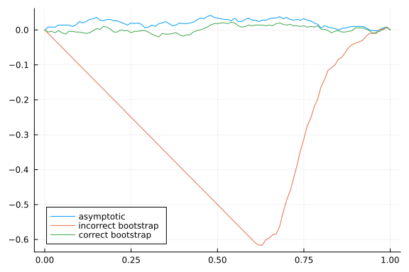
With the same sort of modification the KLM and CLR statistics can also be bootstrapped. All three statistics remain identification robust when bootstrapped. See Kleibergen (2006)¹³ for details.

Single coefficients¶

If we want to construct a confidence interval for a single coefficient, we can apply the bootstrap to a statistic like $\sqrt{n} (\hat{\theta} - \theta_0)$ (or a studentized version of it). Just like in the previous subsection, we must be careful to ensure that the null hypothesis holds in the bootstrapped data. Also, as above, we can do this by subtracting $1/n\sum_i g_i(\hat{\theta})$ from the bootstrapped moments. Thus, one way to bootstrap is $\sqrt{n} (\hat{\theta} - \theta_0)$ is to

• Compute $\hat{\theta}$, $\bar{g}_n(\hat{\theta}) = 1/n\sum_i g_i(\hat{\theta})$
• Draw with replacement $g_i^\ast(\theta)$ from ${g_i(\theta) - \bar{g}n(\hat{\theta})}^n$.
• Compute

$$\hat{\theta}^\ast = \argmin [1/n \sum_i g_i^\ast(\theta)] W_n^\ast(\theta) [1/n \sum g_i^\ast(\theta]$$

• Use distribution of $\sqrt{n} (\hat{\theta}^\ast - \hat{\theta})$ to approximate $\sqrt{n} (\hat{\theta} - \theta_0)$

For some models, the minimazation needed to compute $\hat{\theta}^\ast$ can be very time consuming. Fortunately, it can be avoided. A key step in showing that $\hat{\theta}$ is asymptotically normal is a linearization

$$\sqrt{n}(\hat{\theta} - \theta_0) = -(D'WD)^{-1} (D' W) \frac{1}{\sqrt{n}} \sum_i g_i(\theta_0) + o_p(1)$$

Showing the bootstrap estimator is asymptotically normal conditional on the data involves a similar linearization

$$\sqrt{n}(\hat{\theta}^\ast - \hat{\theta}) = -(\hat{D}'\hat{W}\hat{D})^{-1} (\hat{D}' \hat{W}) \frac{1}{\sqrt{n}} \sum_i g_i^\ast(\hat{\theta}) + o_p(1)$$

This suggests taking

$$\hat{\theta}^\ast = \hat{\theta} + (\hat{D}'\hat{W}\hat{D})^{-1} (\hat{D}' \hat{W}) \frac{1}{\sqrt{n}} \sum_i g_i^\ast(\hat{\theta})$$

instead of re-minimizing.

function gmmVar(θ,gi,W)
  g = gi(θ)
  n = size(g)[1]
  D = ForwardDiff.jacobian(θ->mean(gi(θ),dims=1),θ)
  Σ = cov(gi(θ))
  1/n*inv(D'*W*D)*(D'*W*Σ*W*D)*inv(D'*W*D)
end

function bsweights(n)
  s = sample(1:n,n)
  (x->sum(x.==s)).(1:n)
end


function bootstrapt(θ,gi, W)
  giθ = gi(θ)
  gn = size(giθ)[1]
  D = ForwardDiff.jacobian(θ->mean(gi(θ),dims=1),θ) 
  function bootonce(θ,gi)
    giθ = gi(θ)
    n = size(giθ)[1]
    gn = mean(giθ,dims=1)
    w = bsweights(n)
    giw(θ) = (gi(θ).*w .- gn)
    gmmobj = gmm_objective(giw, W)
    opt1 = optimize(gmmobj, θ, BFGS(), autodiff =:forward)
    θs1 = opt1.minimizer
    θs2 = θ - inv(D'*W*D)*(D'*W*( (mean(giθ.*w,dims=1).-gn)' ))
    [θs1[1] θs2[1]]
  end
  S = 299
  vcat([bootonce(θ,gi) for s in 1:S]...)
end

bootstrapt (generic function with 1 method)

n = 50
k = 2
iv = 3
β0 = ones(k)
π0 = vcat(I,ones(iv-k,k))
ρ = 0.5
data = IVLogitShare(n,β0,π0,ρ)
gi = get_gi(data)
W = I
optres = optimize(gmm_objective(data,W), β0, BFGS(),
                  autodiff = :forward)
θhat = optres.minimizer
θs = bootstrapt(θhat,gi,I)
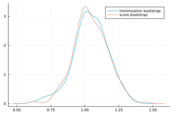
density(θs[:,1], label="minimization bootstrap")
density!(θs[:,2], label="score bootstrap")

function simulatetests()
  data = IVLogitShare(n,β0,π0,ρ)
  gi = get_gi(data)
  W = I
  optres = optimize(gmm_objective(gi,W), β0, BFGS(), autodiff =:forward)
  θhat = optres.minimizer 
  θs = bootstrapt(θhat,gi,I)
  p = mean((θhat[1]-β0[1]).<(θs .- θhat[1]), dims=1)
end

pvals = vcat([simulatetests() for s in 1:300]...)
p = 0:0.01:1.0
fig=plot(p, p->(mean(pvals[:,1].<p)-p),
         label="minimization bootstrap", legend=:best)
plot!(fig,p, p->(mean(pvals[:,2].<p)-p),  label="score bootstrap")
fig

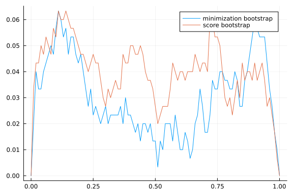
Both versions of the bootstrap appear to work well enough here. Note that neither one is robust to identification problems. Inference on a subset of parameters while remaining robust to identification problems is somewhat of an open problem. Various conservative approaches are available, the simplest of which is to just take projections of the AR, KLM, or CLR confidence sets. There are also more powerful approaches for situations where you know which parameters are strongly vs weakly identified.

References¶