This work is licensed under a Creative Commons Attribution-ShareAlike 4.0 International License

About this document¶

This document was created using Weave.jl. The code is available in on github. The same document generates both static webpages and associated jupyter notebook.

$\def\indep{\perp\!\!\!\perp} \def\Er{\mathrm{E}} \def\R{\mathbb{R}} \def\En{{\mathbb{E}_n}} \def\Pr{\mathrm{P}} \newcommand{\norm}[1]{\left\Vert {#1} \right\Vert} \newcommand{\abs}[1]{\left\vert {#1} \right\vert} \DeclareMathOperator*{\argmax}{arg\,max} \DeclareMathOperator*{\argmin}{arg\,min}$

Introduction¶

This document is a companion to my “Machine learning in economics”. Those notes discuss the recent use of machine learning in economics, with a focus on lasso and random forests. The code in those notes is written in R. This document will look at similar code in Julia.

RCall¶

If you want to use the methods of Chernozhukov and coauthors implements in the R packaga Chernozhukov, Victor, Chris Hansen, and Martin Spindler, “[hdm]{.nocase}: High-dimensional metrics,” R Journal, 8 (2016), 185–199. or the methods of Athey and coauthors implemented in the R package Tibshirani, Julie, Susan Athey, Stefan Wager, Rina Friedberg, Luke Miner, and Marvin Wright, “Grf: Generalized random forests (beta),” (2018). , then it makes sense to use the R pacakge. You could simply write all your code in R. However, if you prefer using Julia, you can just call the necessary R functions with RCall.jl.

Here, we load the pipeline data used in the machine learning methods notes, and do some cleaning in Julia.

using RCall, DataFrames, Missings, Statistics
R"load(paste($(docdir),\"/rmd/pipelines.Rdata\",sep=\"\"))"
println(R"ls()")
data = @rget data # data on left is new Julia variable, data on right is the one in R
println(R"summary(data[,1:5])")
println(describe(data[:,1:5]))
for c in 59:107 # columns of state mileage, want missing->0
  replace!(x->(ismissing(x) || isnan(x)) ? 0.0 : x, data[!,c])
end
println(describe(data[:,59:65]))

RObject{StrSxp}
[1] "#JL"  "data"

RObject{StrSxp}
 respondent_id     report_yr      report_prd     major        
 Min.   :  1.0   Min.   :1991   Min.   :12     Mode :logical  
 1st Qu.: 64.0   1st Qu.:1997   1st Qu.:12     FALSE:1192     
 Median :148.0   Median :2003   Median :12     TRUE :2797     
 Mean   :184.3   Mean   :2003   Mean   :12     NA's :2180     
 3rd Qu.:214.0   3rd Qu.:2010   3rd Qu.:12                    
 Max.   :745.0   Max.   :2016   Max.   :12                    
                                NA's   :3371                  
                             respondent_name
 Centra Pipelines Minnesota Inc.     :  22  
 Tuscarora Gas Transmission Company  :  22  
 Eastern Shore Natural Gas Company   :  22  
 Kern River Gas Transmission Company :  21  
 National Fuel Gas Supply Corporation:  21  
 (Other)                             :2938  
 NA's                                :3123

5×7 DataFrame
 Row │ variable         mean      min                                median  max                                nmissing  eltype
     │ Symbol           Union…    Any                                Union…  Any                                Int64     Type
─────┼──────────────────────────────────────────────────────────────────────────────────────────────────────────────────────────────────────────────────────
   1 │ respondent_id    184.3     1                                  148.0   745                                       0  Int64
   2 │ report_yr        2003.49   1991                               2003.0  2016                                      0  Int64
   3 │ report_prd       12.0      12                                 12.0    12                                     3371  Union{Missing, Int64}
   4 │ major            0.701178  false                              1.0     true                                   2180  Union{Missing, Bool}
   5 │ respondent_name            Algonquin Gas Transmission Compa…          Southern Natural Gas Company    …      3123  Union{Missing, CategoricalValue{…
7×7 DataFrame
 Row │ variable        mean        min      median   max       nmissing  eltype
     │ Symbol          Float64     Float64  Float64  Float64   Int64     Union
─────┼───────────────────────────────────────────────────────────────────────────────────────────
   1 │ North Carolina  0.00358525      0.0      0.0  1.0              0  Union{Missing, Float64}
   2 │ Tennessee       0.0061488       0.0      0.0  0.635202         0  Union{Missing, Float64}
   3 │ Virginia        0.00552028      0.0      0.0  1.0              0  Union{Missing, Float64}
   4 │ Illinois        0.0134891       0.0      0.0  1.0              0  Union{Missing, Float64}
   5 │ Indiana         0.0058707       0.0      0.0  0.550302         0  Union{Missing, Float64}
   6 │ Kentucky        0.0133474       0.0      0.0  1.0              0  Union{Missing, Float64}
   7 │ Gulf of Mexico  0.0140981       0.0      0.0  0.825409         0  Union{Missing, Float64}

Suppose we want to estimate the coefficient on transPlant (capital) in a partially linear model with transProfit (profit) as the outcome. This can be done with the R function hdm::rlassoEffects.

R"library(hdm)"
completedata = dropmissing(data,[1:10..., 59:122...], disallowmissing=true)
y = completedata[!,:transProfit]
inc = .!isnan.(y)
y = y[inc]
X = completedata[inc,[6:7..., 59:121...]]
cols = [std(X[!,c])>0 for c in 1:ncol(X)]
X = X[:,cols]
est = R"rlassoEffects($(X), $(y), index=c(1:2))"
R"summary($est)"

RObject{VecSxp}
[1] "Estimates and significance testing of the effect of target variables"
                      Estimate. Std. Error t value Pr(>|t|)    
transPlant_bal_end_yr  0.034434   0.008878   3.879 0.000105 ***
transPlant_bal_beg_yr  0.086580   0.009383   9.228  < 2e-16 ***
---
Signif. codes:  0 ‘***’ 0.001 ‘**’ 0.01 ‘*’ 0.05 ‘.’ 0.1 ‘ ’ 1

MLJ.jl¶

MLJ.jl is a machine learning framework for Julia. It gives a unified interface for many machine learning algorithms and tasks. Similar R packages include caret and MLR. scikit-learn is a similar Python package.

For more information on MLJ see

You can see a list of models registered to work with MLJ.jl on github, or by calling MLJ::models().

using MLJ
models()

239-element Vector{NamedTuple{(:name, :package_name, :is_supervised, :abstr
act_type, :constructor, :deep_properties, :docstring, :fit_data_scitype, :h
uman_name, :hyperparameter_ranges, :hyperparameter_types, :hyperparameters,
 :implemented_methods, :inverse_transform_scitype, :is_pure_julia, :is_wrap
per, :iteration_parameter, :load_path, :package_license, :package_url, :pac
kage_uuid, :predict_scitype, :prediction_type, :reporting_operations, :repo
rts_feature_importances, :supports_class_weights, :supports_online, :suppor
ts_training_losses, :supports_weights, :tags, :target_in_fit, :transform_sc
itype, :input_scitype, :target_scitype, :output_scitype)}}:
 (name = ABODDetector, package_name = OutlierDetectionNeighbors, ... )
 (name = ABODDetector, package_name = OutlierDetectionPython, ... )
 (name = ARDRegressor, package_name = MLJScikitLearnInterface, ... )
 (name = AdaBoostClassifier, package_name = MLJScikitLearnInterface, ... )
 (name = AdaBoostRegressor, package_name = MLJScikitLearnInterface, ... )
 (name = AdaBoostStumpClassifier, package_name = DecisionTree, ... )
 (name = AffinityPropagation, package_name = Clustering, ... )
 (name = AffinityPropagation, package_name = MLJScikitLearnInterface, ... )
 (name = AgglomerativeClustering, package_name = MLJScikitLearnInterface, .
.. )
 (name = AutoEncoder, package_name = BetaML, ... )
 ⋮
 (name = TomekUndersampler, package_name = Imbalance, ... )
 (name = UnivariateBoxCoxTransformer, package_name = MLJTransforms, ... )
 (name = UnivariateDiscretizer, package_name = MLJTransforms, ... )
 (name = UnivariateFillImputer, package_name = MLJTransforms, ... )
 (name = UnivariateStandardizer, package_name = MLJTransforms, ... )
 (name = UnivariateTimeTypeToContinuous, package_name = MLJTransforms, ... 
)
 (name = XGBoostClassifier, package_name = XGBoost, ... )
 (name = XGBoostCount, package_name = XGBoost, ... )
 (name = XGBoostRegressor, package_name = XGBoost, ... )

To use these models, you need the corresponding package to be installed and loaded. The @load macro will load the needed package(s) for any model.

Lasso = @load LassoRegressor pkg=MLJLinearModels

import MLJLinearModels ✔
MLJLinearModels.LassoRegressor

Let’s fit lasso to the same pipeline data as above.

lasso = machine(Lasso(lambda=1.0), X, y)
train,test = partition(eachindex(y), 0.6, shuffle=true)
fit!(lasso, rows=train)
yhat = predict(lasso, rows=test)
println(yhat[1:10])
println("MSE/var(y) = $(mean((y[test].-yhat).^2)/var(y[test]))")

[0.0, 0.0, 0.0, 0.0, 0.0, 0.0, 0.0, 0.0, 0.0, 0.0]
MSE/var(y) = 1.5024909580796766

That doesn’t look very good. All the predictions are zero. This could happen when the regularization parameter, lambda, is too large. However, in this case the problem is something else. The warning messages indicate numeric problems when minimizing the lasso objective function. This can happen when X is poorly scaled. The algorithm used to compute the lasso estimates works best when the coefficients are all roughly the same scale. The existing X’s have wildly different scales, which causes problems. This situation is common, so MLJ.jl has functions to standardize variables. It is likely that the hdm package in R does something similar internally.

lasso_stdx = Pipeline(Standardizer(),
                      Lasso(lambda=1.0*std(y[train]),
                            solver=MLJLinearModels.ISTA(max_iter=10000))
                      )
m = machine(lasso_stdx, X, y)
fit!(m, rows=train, force=true)
yhat = predict(m , rows=test)
println("MSE/var(y) = $(mean((y[test].-yhat).^2)/var(y[test]))")

# Get the fitted coefficients
coef = fitted_params(m).lasso_regressor.coefs
intercept = fitted_params(m).lasso_regressor.intercept
sum(abs(c[2])>1e-8 for c in coef) # number non-zero

MSE/var(y) = 0.9994939567244565
0

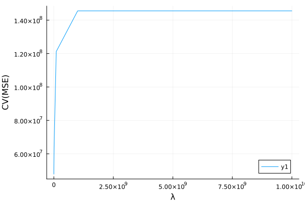
If we want to tune lambda using cross-validation, we can use the range and TunedModel functions.

r = range(lasso_stdx, :(lasso_regressor.lambda), lower=1e1, upper=1e10, scale=:log)
t=TunedModel(model=lasso_stdx,
             resampling=CV(nfolds=5),
             tuning=Grid(resolution=10),
             ranges=r,
             measure=rms)
m = machine(t, X, y)
fit!(m, rows=train, verbosity=1)
yhat = predict(m , rows=test)
println("MSE/var(y) = $(mean((y[test].-yhat).^2)/var(y[test]))")

MSE/var(y) = 0.15134783267464927

using Plots
cvmse = report(m).plotting.measurements
λ = Float64.(report(m).plotting.parameter_values[:])
s = sortperm(λ)
plot(λ[s], cvmse[s], xlab="λ", ylab="CV(MSE)")

Flux.jl¶

Flux.jl is another Julia package for machine learning. It seems to be emerging as the leading Julia package for neural networks and deep learning, but other machine learning models can also be implemented using Flux.jl.

Let’s create a lasso model in Flux.jl.

using Flux, LinearAlgebra
# Scale the variables
Xstd = Flux.normalise(Matrix(X), dims=1)
X_train = Xstd[train,:]
X_test = Xstd[test,:]
yscale = std(y[train])
ymean = mean(y[train])
ystd = (y .- ymean)./yscale
y_train = ystd[train]
y_test = ystd[test]

# Set up the model parameters and initial values
βols = (X_train'*X_train) \ (X_train'*(y_train .- mean(y_train)))
β = zeros(ncol(X))
b = mean(y_train)

# Define the loss function
ψ = ones(length(β))
λ = 2.0

mutable struct LinearModel
  β::Vector{Float64}
  b::Float64
end

pred(m::LinearModel,x) = m.b .+ x*m.β
mse(m::LinearModel,x,y) = mean( (pred(m,x) .- y).^2 )
penalty(m::LinearModel,y) = λ/length(y)*norm(ψ.*m.β,1)
loss(m::LinearModel,x,y) =  mse(m,x,y) + penalty(m,y)
m = LinearModel(β,b)
@show loss(m,X_train,y_train)

# minimize loss
maxiter=2000
obj = zeros(maxiter)
mse_train = zeros(maxiter)
mse_test = zeros(maxiter)
opt = Flux.setup(Flux.AMSGrad(), m)
import ProgressMeter: @showprogress
@showprogress for i in 1:maxiter
  Flux.train!(loss, m, [(X_train, y_train)], opt)
  mse_train[i] = mse(m,X_train,y_train)
  mse_test[i] = mse(m,X_test, y_test)
  obj[i] = loss(m,X_train,y_train)
end
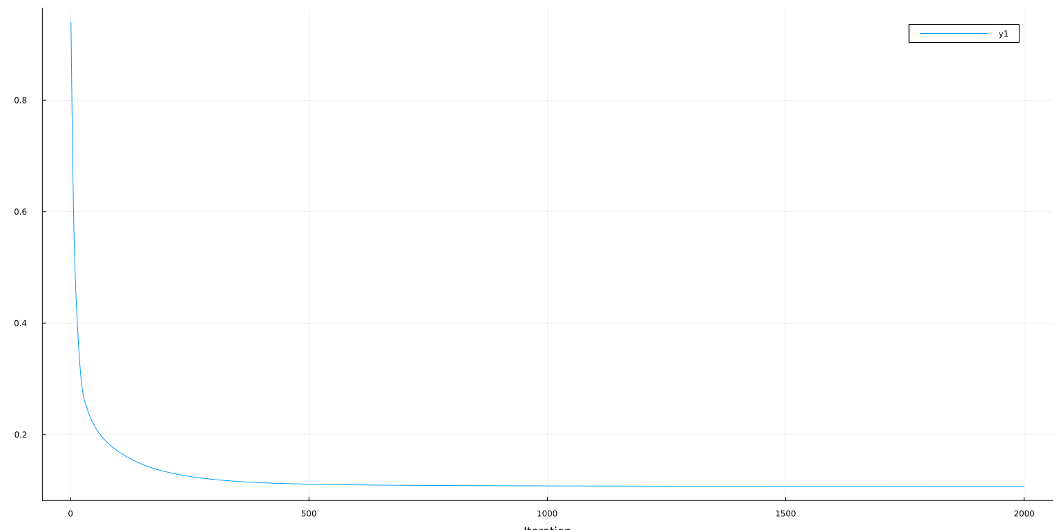
lo = 1
hi = 2000
plot(obj[lo:hi], ylab="Loss=MSE + λ/n*||β||₁", xlab="Iteration")

loss(m, X_train, y_train) = 0.9986320109439124

plot(lo:hi, [mse_train[lo:hi] mse_test[lo:hi]], ylab="MSE", xaxis=("Iteration"), lab=["Train" "Test"])

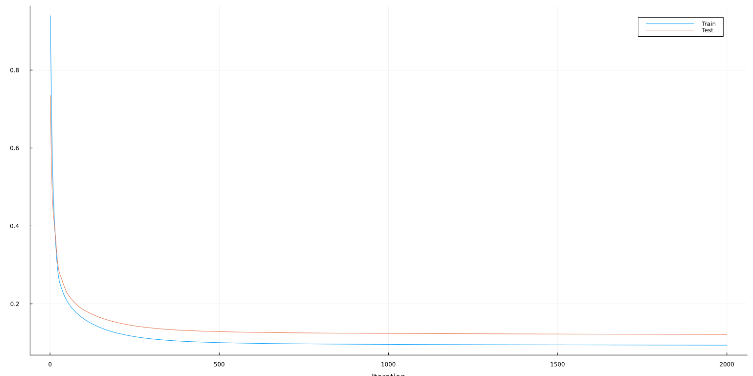
The minimization methods in Flux.train! are all variants of gradient descent. Each call to Flux.train! runs one iteration of the specified solver. To find a local minimum, Flux.train! can be called repeatedly until progress stops. The above loop is a simple way to do this. The @epoch macro can also be useful.

Gradient descent works well for neural networks, but is not ideal for Lasso. Without further adjustment, gradient descent gets stuck in a cycle as jumps from one side of the other of the absolute value in the lasso penalty. Nonetheless, the results are near the true minimum, even though it never exactly gets there.

Lux.jl¶

A promising alternative to Flux.jl is Lux.jl.¹ Lux.jl and Flux.jl share many features and backend code. Lux.jl has a more function focused interface with explicit parameter passing. This is a more “Julian” style of programming.²

For comparison, let’s implement the same Lasso model in Lux.

import Lux # Lux shares many function names with Flux, so import instead of using to avoid confusion
import Random, Zygote
using Test
# Seeding
rng = Random.default_rng()
Random.seed!(rng, 0)

# define the model
X_train = Matrix(X)[train,:]
X_test = Matrix(X)[test,:]
y_train = y[train]
y_test = y[test]
function standardizer(xtrain)
  m = std(xtrain, dims=1)
  s = std(xtrain, dims=1)
  (x->(x .- m)./s , xs->xs.*s .+ m)
end
stdizex, _ = standardizer(X_train)
stdizey, unstdizey = standardizer(y_train)
@test unstdizey(stdizey(y_test)) ≈ y_test

ys = stdizey(y_train)
Xs = stdizex(X_train)
# Set up the model parameters and initial values
βols = (Xs'*Xs) \ (Xs'*(ys .- mean(ys)))
b = [mean(ys)]

m = Lux.Chain(X->stdizex(X)',
              Lux.Dense(size(X_train,2), 1)
              )
ps, st = Lux.setup(rng, m)
ps.layer_2.weight .= βols'
ps.layer_2.bias .= b

mse(m, ps, st, X, y) = mean(abs2, m(X, ps, st)[1]' .- stdizey(y))
mseraw(m,ps,st,X,y) = mean(abs2, unstdizey(m(X, ps, st)[1]') .- y)
ℓ = let λ = 2.0, ψ = ones(size(βols')), st=st
  penalty(ps,y) = λ/length(y)*norm(ψ.*ps.layer_2.weight,1)
  loss(ps, X, y, m) = mse(m, ps, st, X, y) + penalty(ps,y)
end

@show ℓ(ps,X_train,y_train,m)

# minimize loss
import Optimisers

function train_model(m, initial_params, st; maxiter=2000)
    opt = Optimisers.AMSGrad()
    ps = initial_params
    optstate = Optimisers.setup(opt, ps)

    obj = zeros(maxiter)
    mse_train = zeros(maxiter)
    mse_test = zeros(maxiter)
    @showprogress for i in 1:maxiter
        # Compute the gradient
        gs = Zygote.gradient(ps->ℓ(ps, X_train, y_train, m), ps)[1]
        # Perform parameter update
        optstate, ps = Optimisers.update(optstate, ps, gs)
        mse_train[i] = mse(m, ps, st, X_train,y_train)
        mse_test[i] = mse(m, ps, st, X_test, y_test)
        obj[i] = ℓ(ps,X_train,y_train,m)
    end
    return(ps, mse_train, mse_test, obj)
end
ps, mse_train, mse_test, obj = train_model(m, ps, st)
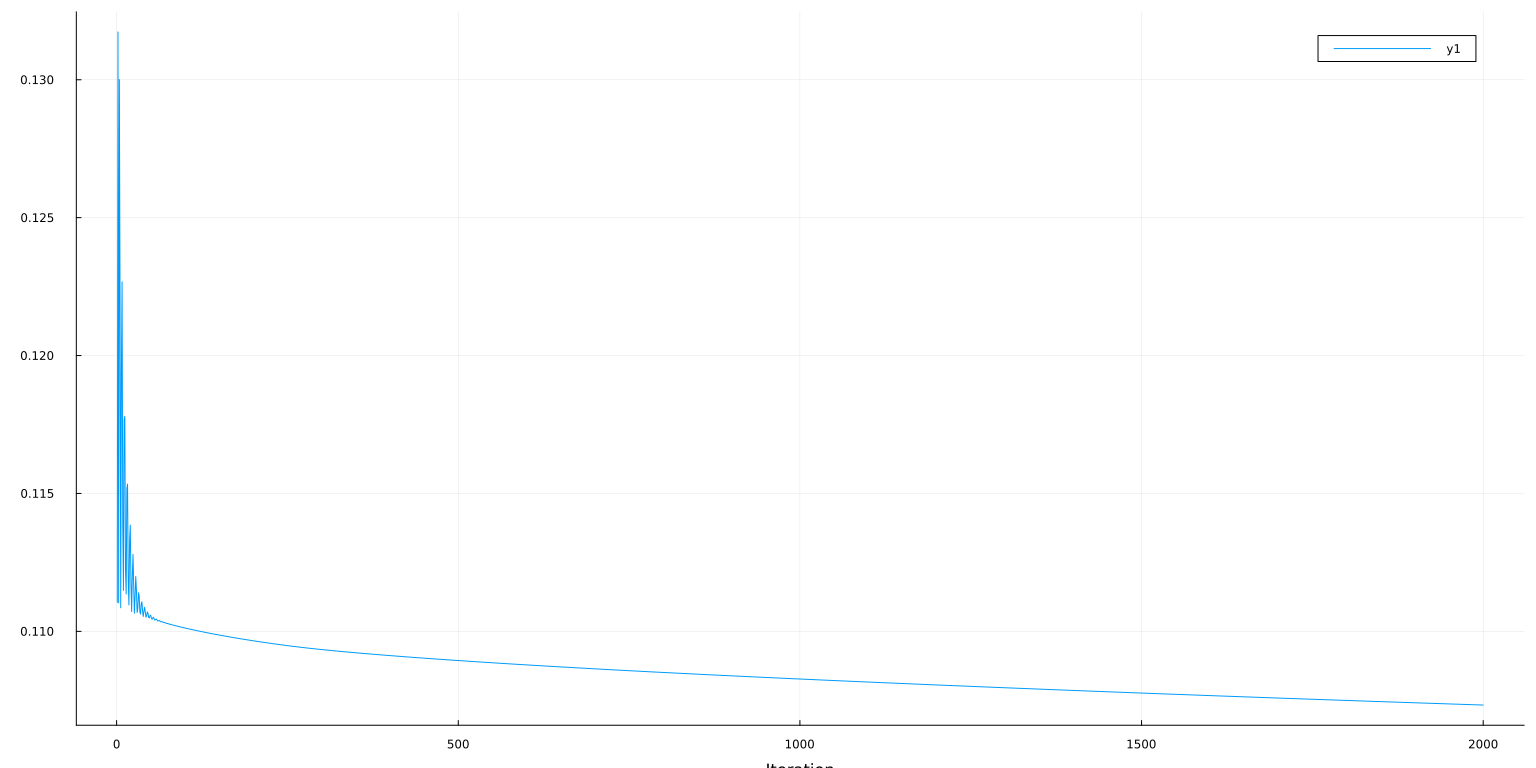
lo = 1
hi = 2000
plot(lo:hi,obj[lo:hi], ylab="Loss=MSE + λ/n*||β||₁", xlab="Iteration")

ℓ(ps, X_train, y_train, m) = 0.11116189450789928

plot(lo:hi, [mse_train[lo:hi] mse_test[lo:hi]], ylab="MSE", xaxis=("Iteration"), lab=["Train" "Test"])

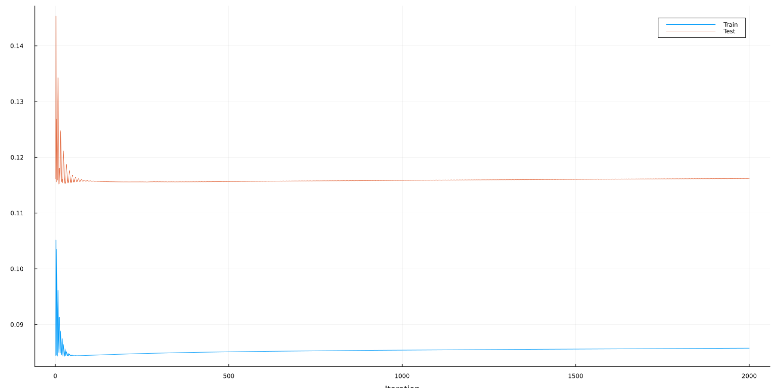
Additional Resources¶

(Klok and Nazarathy 2019)³ Statistics with Julia:Fundamentals for Data Science, MachineLearning and Artificial Intelligence

References¶

These notes were originally written before Lux.jl existed. If I were starting over, I would use Lux.jl instead of Flux.jl. ↩
Flux.jl drew inspiration for its interface from Tensorflow and PyTorch. Implicit parameters makes some sense in an object oriented language like Python, but it is not the most natural style for Julia. ↩
Klok, Hayden, and Yoni Nazarathy, “Statistics with julia:fundamentals for data science, MachineLearning and artificial intelligence,” (DRAFT, 2019). ↩

Keys	Action
`?`	Open this help
`n`	Next page
`p`	Previous page
`s`	Search