This work is licensed under a Creative Commons Attribution-ShareAlike 4.0 International License

About this document¶

This document was created using Weave.jl. The code is available in on github. The same document generates both static webpages and associated jupyter notebook.

$\def\indep{\perp\!\!\!\perp} \def\Er{\mathrm{E}} \def\R{\mathbb{R}} \def\En{{\mathbb{E}_n}} \def\Pr{\mathrm{P}} \newcommand{\norm}[1]{\left\Vert {#1} \right\Vert} \newcommand{\abs}[1]{\left\vert {#1} \right\vert} \DeclareMathOperator*{\argmax}{arg\,max} \DeclareMathOperator*{\argmin}{arg\,min}$

Introduction¶

The previous notes discussed single layer neural networks. These notes will look at multiple layer networks.

Additional Reading¶

(Goodfellow, Bengio, and Courville 2016)¹ Deep Learning
Knet.jl documentation especially the textbook
(Klok and Nazarathy 2019)² Statistics with Julia:Fundamentals for Data Science, MachineLearning and Artificial Intelligence
(Farrell, Liang, and Misra 2018)³ “Deep Neural Networks for Estimation and Inference”

Multiple Layer Neural Networks¶

A multiple layer feed forward neural network (aka a multi-layer perception) connects many single layer networks. A multi-layer perceptron can be written recursively. The outermost layer of a multi-layer perception looks like a generalized linear model: $\hat{f}(x) = \psi_L(x_L' w_L+ b_L)$ where $x_L, w_L \in \R^{H_L}$, $b_L \in \R$, and $\psi_L: \R \to \R$. For regression problems, $\psi_L$ is typically the identity function.

In a generalized linear model, $x_L$ would be data. In a multilayer network, $x_L \in \R^{H_{L}}$ is the output of a previous layer. Specificaly, for $k \in { 1, ...., H_L}$, $x_{k,L} = \psi_{k, L-1}(x_{L-1}'w_{k,L-1} + b_{k,L-1})$ where $x_{L-1}, w_{L-1} \in \R^{H_{L-1}}$, $b_{L-1} \in \R$, and $\psi_{k,L-1}: \R \to \R$. This continues recursively until $x_0 = x \in \R^d$ is the data.

$L$ is the depth of the network.

::: {.alert .alert-danger} When $L$ is sufficiently large, you have a deep neural network, and can attract grant money by calling your research deep learning and/or AI. :::

$H_\ell$ is the width of layer $\ell$. Following (Farrell, Liang, and Misra 2018)³, we will let $U = \sum_{\ell=1}^L H_\ell$ denote the number of units. The number of parameters is $W = \sum_{\ell=1}^L (H_{\ell-1}+1) H_\ell$ where $H_0 = d$ is the dimension of the data.

In most applications, the activation within a layer is the same for each unit, i.e. $\psi_{k,\ell}$ does not vary with $k$. In large networks and/or with large datasets, activation functions are usually (leaky) rectified linear to allow faster computation.

The combination of depths ($L$), width ($H_\ell$), and activation functions ($\psi$) are collectively referred to as the network architecture.

First Example¶

As a starting example, here is some code that fits a multi-layer network to the same simulated data as in the notes on single layer networks.

Simulating data and setting up.

using Plots, Flux, Statistics, ColorSchemes
# some function to estimate
_f(x) = sin(x^x)/2^((x^x-π/2)/π)
function simulate(n,s=1)
  x = rand(n,1).*π
  y = _f.(x) .+ randn(n).*s
  (x,y)
end
x, y = simulate(1000, 0.5)
xt = reshape(x, 1, length(x))
yt = reshape(y, 1, length(y))
xg = 0:0.01:π
cscheme = colorschemes[:BrBG_4];
dimx = 1
xt = reshape(Float32.(x), 1, length(x))
yt = reshape(Float32.(y), 1, length(y))

1×1000 Matrix{Float32}:
 0.927618  -0.220508  0.632587  1.09905  …  0.556763  0.980371  0.651816

We now define our models. The second model is a multi-layer network with 3 layers each of width 3. The first model is a single-layer network with width 15. This makes the total number of parameters in the two networks equal. For both networks we normalise $x$ and then use Flux’s default initial values (these set $b=0$ and $w$ random).

mlps = [ Chain(x->Flux.normalise(x, dims=2),
                 Dense(dimx, 15, Flux.leakyrelu),
                 Dense(15, 1)),
           Chain(x->Flux.normalise(x, dims=2),
                 Dense(dimx, 3, Flux.leakyrelu),
                 Dense(3, 3, Flux.leakyrelu),
                 Dense(3, 3, Flux.leakyrelu),
                 Dense(3, 1))
           ]


figs = Array{typeof(plot(0)),1}(undef,length(mlps))
initmfigs = Array{typeof(plot(0)),1}(undef,length(mlps))

for r in eachindex(mlps)
  m = mlps[r]
  println("Model $r = $m")
  nparm = sum([length(m[i].weight) + length(m[i].bias) for i in 2:length(m)])
  println(" $nparm parameters in $(length(m)-1) layers")
  initmfigs[r] = plot(xg, m[1:(end-1)](xg')', lab="", legend=false)
  figs[r]=plot(xg, _f.(xg), lab="", title="Model $r", color=:red)
  figs[r]=scatter!(x,y, alpha=0.4, markersize=1, markerstrokewidth=0, lab="")
  maxiter = 2000
  opt = Flux.setup(Flux.AMSGrad(),m)
  @time for i = 1:maxiter
      Flux.train!((m,x,y)->Flux.mse(m(x),y), m,
                  #[(xt[:,b], yt[:,b]) for b in Base.Iterators.partition(1:length(yt), 500)],
                [(xt, yt)],
                opt) #,
                #cb = Flux.throttle(()->@show(Flux.mse(m(xt),yt)),100))
    if i==1 || (i % (maxiter ÷ 10)==0)
      l=Flux.mse(m(xt), yt)
      println("Model $r, $i iterations, loss=$l")
      yg = m(xg')'
      loc=Int64.(ceil(length(xg)*i/maxiter))
      figs[r]=plot!(xg,yg, lab="", color=get(cscheme, i/maxiter), alpha=1.0,
                    annotations=(xg[loc], yg[loc],
                                 Plots.text("i=$i", i<maxiter/2 ? :left : :right, pointsize=10,
                                            color=get(cscheme, i/maxiter)) )
                    )
    end
  end
  display(figs[r])
end

Model 1 = Chain(#3, Dense(1 => 15, leakyrelu), Dense(15 => 1))
 46 parameters in 2 layers
Model 1, 1 iterations, loss=0.74293023
Model 1, 200 iterations, loss=0.27535582
Model 1, 400 iterations, loss=0.2599157
Model 1, 600 iterations, loss=0.2539969
Model 1, 800 iterations, loss=0.2523616
Model 1, 1000 iterations, loss=0.25194454
Model 1, 1200 iterations, loss=0.25175378
Model 1, 1400 iterations, loss=0.2517021
Model 1, 1600 iterations, loss=0.25168243
Model 1, 1800 iterations, loss=0.25167215
Model 1, 2000 iterations, loss=0.25166646
 13.236452 seconds (54.92 M allocations: 3.049 GiB, 2.04% gc time, 98.65% c
ompilation time)
Model 2 = Chain(#5, Dense(1 => 3, leakyrelu), Dense(3 => 3, leakyrelu), Den
se(3 => 3, leakyrelu), Dense(3 => 1))
 34 parameters in 4 layers
Model 2, 1 iterations, loss=0.95467716
Model 2, 200 iterations, loss=0.45980266
Model 2, 400 iterations, loss=0.32117203
Model 2, 600 iterations, loss=0.27392912
Model 2, 800 iterations, loss=0.25515068
Model 2, 1000 iterations, loss=0.25385037
Model 2, 1200 iterations, loss=0.25377107
Model 2, 1400 iterations, loss=0.25375405
Model 2, 1600 iterations, loss=0.25374243
Model 2, 1800 iterations, loss=0.25372878
Model 2, 2000 iterations, loss=0.25371048
  0.985196 seconds (5.54 M allocations: 623.481 MiB, 8.40% gc time, 73.96% 
compilation time)

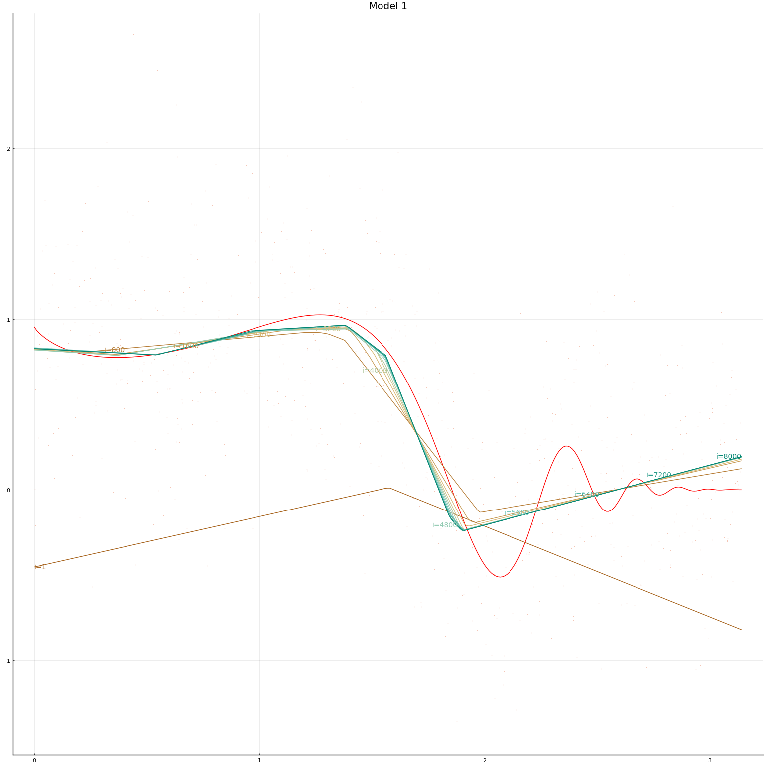
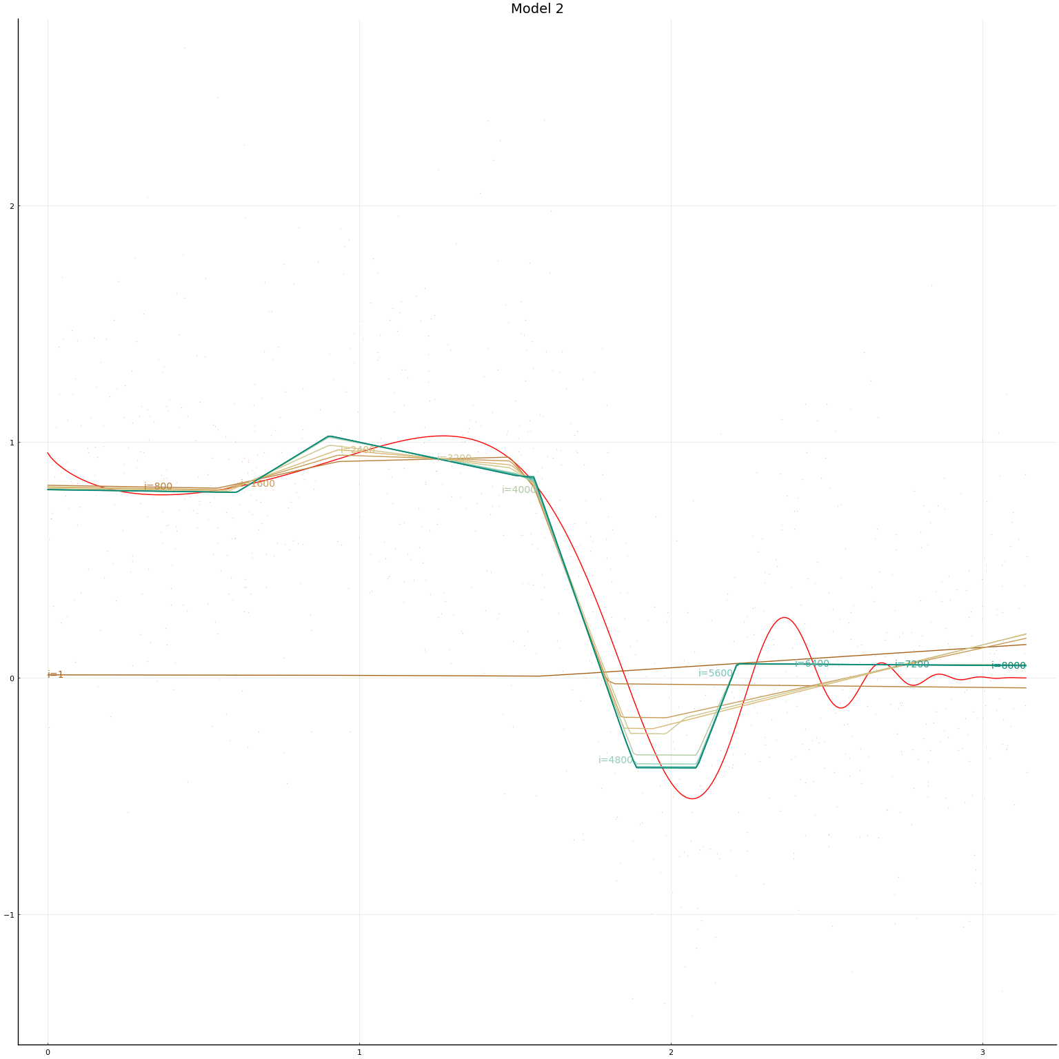
In this simulation setup, the performance of the two network architectures is hard to distinguish. The multi-layer network takes a bit longer to train. Depending on the randomly simulated data, and randomly drawn initial values, either model might achieve lower in-sample MSE.

Image Classification: MNIST¶

MNIST is a database of images of handwritten digits. MNIST is a common machine learning benchmark. Given a handwritten digit, we want to classify it is a 0, 1, …, or 9. You can try a demo of a MNIST classifier trained in Flux here.

Multilayer feed forward networks generally have good, but not quite state-of-the-art performance in image classification. Nonetheless, this will hopefully serve as a good example.

::: {.alert .alert-danger} The code in this section was adapted from the Flux model zoo. :::

First we load some packages and download the data.

using Flux, Statistics
using Flux: onehotbatch, onecold, crossentropy, throttle
using Base.Iterators: repeated
using CUDA
using JLD2
using MLDatasets

# load training set
train_x, train_y = MNIST(split=:train)[:]

# load test set
test_x,  test_y  = MNIST(split=:test)[:]

modeldir = normpath(joinpath(docdir,"jmd","models"))
if !isdir(modeldir)
  mkdir(modeldir)
end

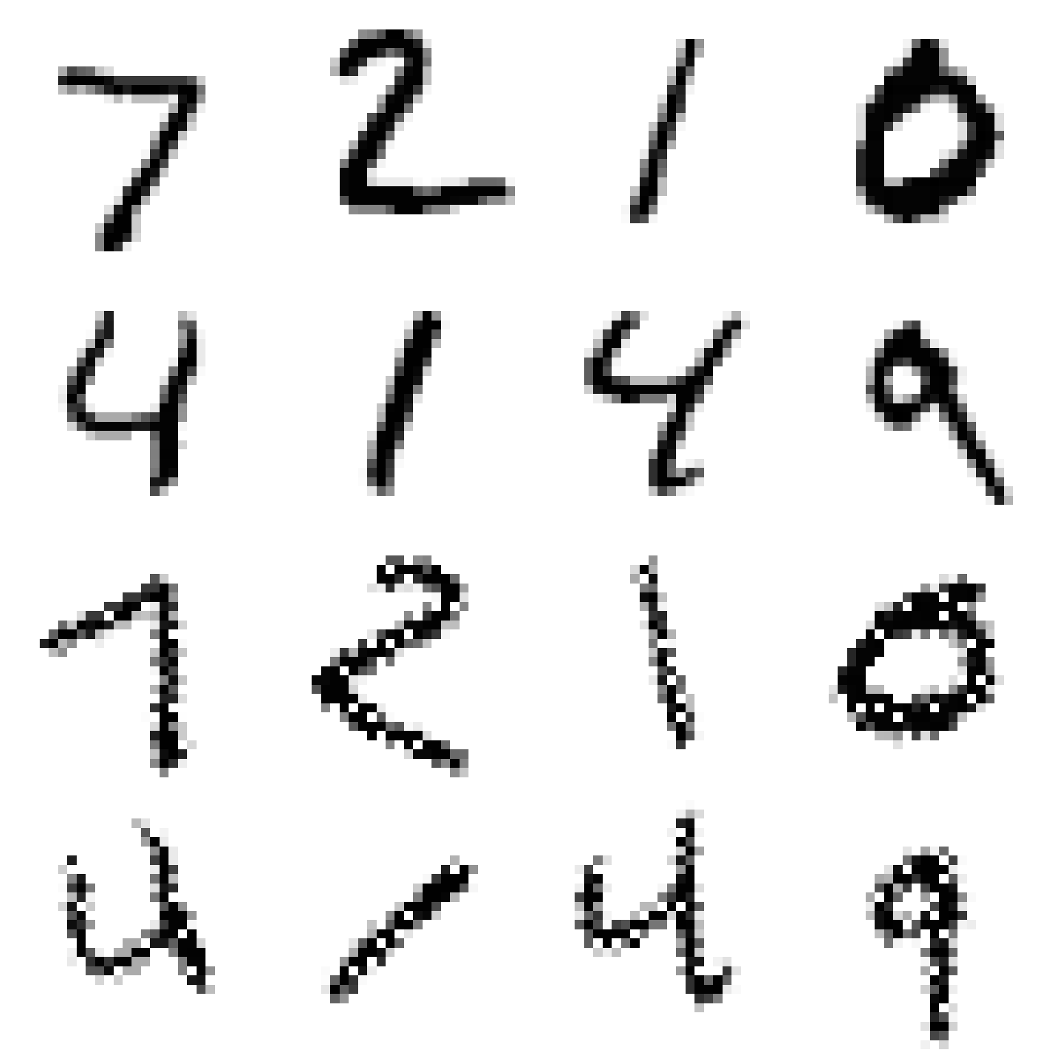
Let’s look at some of the images.

# Previously MNIST was provided in the Flux package in a different format.
# To keep code compatible, we convert to the old format
imgs = vcat([Gray.(1 .-train_x[:,:,i]') for i ∈ 1:size(train_x,3)],
            [Gray.(1 .-test_x[:,:,i]') for i ∈ 1:size(test_x,3)])
labels = vcat(train_y, test_y)
idx = rand(1:length(imgs), 16)
plot([plot(imgs[i], title="$(labels[i])", aspect_ratio=:equal, axis=false, ticks=false) for i in idx]...)

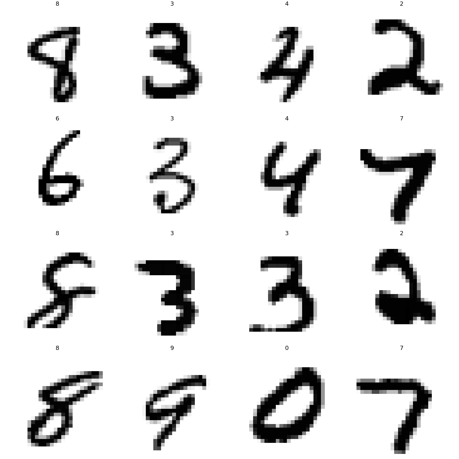
The images are 28 by 28 pixels.

Continue processing the data

# Stack images into one large batch
X = Float32.(reshape(train_x, size(train_x,1)*size(train_x,2), size(train_x,3))) |> gpu;
tX = Float32.(reshape(test_x, size(train_x,1)*size(train_x,2), size(test_x,3))) |> gpu;
# One-hot-encode the labels
Y = onehotbatch(train_y, 0:9) |> gpu;
tY = onehotbatch(test_y, 0:9) |> gpu;

One hot encoding is what the machine learning world calls creating dummy variables from a categorical variable.

Single Layer Classification¶

Now we define our neural network. To begin with we will look at single hidden layer with a multinomial logit output layer. The function that gives choice probabilities in a multinomial logit model is called the softmax function. That is, $softmax(x_1, ..., x_k) = \left( \frac{e^{x_1}}{\sum_{j=1}^k e^{x_i}}, \frac{e^{x_2}}{\sum_{j=1}^k e^{x_i}}, ..., \frac{e^{x_k}}{\sum_{j=1}^k e^{x_i}} \right)$

mstart = Chain(
  Dense(28^2, 32, relu),
  Dense(32, 10))

Chain(
  Dense(784 => 32, relu),               # 25_120 parameters
  Dense(32 => 10),                      # 330 parameters
)                   # Total: 4 arrays, 25_450 parameters, 99.617 KiB.

In this example, we are working on a classification problem; we are trying to predict a discrete outcome instead of a continuous one. The output of the network above are probabilities that an image represents each of the ten digits. That is, we forming conditional probability, or the likelihood, of $y$ given $x$. In this situation, maximum likelihood is a natural estimator. For discrete $y$ (like we have here), the log likelihood is equal to minus the cross-entropy, so this is what we use as our loss function.

loss(m, x, y) = Flux.logitcrossentropy(m(x), y)

loss (generic function with 1 method)

Since cross-entropy or log likelihood are difficult to interpret, we might want a more intuitive measure of our model’s performance. For classification accuracy is the portion of predictions that are correct.

::: {.alert .alert-danger} Other measures of classification performance

For this application accuracy is likely sufficient, but in some situations (including rare outcomes or when we weight differently type I and type II errors) accuracy is not a sufficient measure of a classifier’s performance. There are variety of other measures, such as precision, recall, and AUC. See Batista, Quentin, Chase Coleman, Spencer Lyon, Jesse Perla, Thomas Sargent, Paul Schrimpf, and Natasha Watkins, “Classification,” 2019. for more information. :::

function accuracy(m, x, y)
  # onecold(m(x)) results in very slow code for large x, so we avoid it
  coldx = vec(map(x->x[1], argmax(m(x), dims=1)))
  coldy = onecold(y)
  return(mean(coldx.==coldy))
end;

onecold is the inverse of one-hot-encoding; onecold transforms a matrix of dummy varibles (or probabilities) into an integer (the one with the highest probability in the case of m(x)).

# gradient descent steps using the full X and Y to compute gradients
Xsmall=X[:,1:2000]
Ysmall=Y[:,1:2000] # accuracy is slower, so only compute on subset of data
function evalcb(m)
  l = loss(m, X, Y)
  if isnan(l)
    @show (l)
  else
    @show (l, accuracy(m, Xsmall,Ysmall), accuracy(m, tX,tY))
  end
end;

::: {.alert .alert-danger} Optimizers

Neural networks are usually trained using a variant of gradient descent for optimization. Recall that gradient descent searches for the minimum by taking steps of the form: $\theta_{new} = \theta - \eta Df_{\theta}$ where $\eta$ is a step size or learning rate parameter that gets adjusted depending on algorithm progress. There are many variants of gradient descent available in Flux.jl and they differ in how they adjust the learning rate, $\eta$, and other details. Some algorithms add “momentum” to avoid the long narrow valley problem we saw in the banana function example in the optimization notes. Ruder (2016) gives a nice overview of various forms of gradient descent. :::

Since Flux.train! might run for a long time, it allows us to pass a “callback” function that gets evaluated every iteration. Here, this function is just used to monitor progress. In some situations, we might also want to use the callback function to save intermediate results to disk in case the computation gets interrupted before completion. The Flux.throttle function can be used to prevent the call-back function from being evaluated too often. The code below makes evalcb get evaluated at most once every 10 seconds.

Flux.train does not automatically check that the optimizer is making progress. With too large of a step size, gradient descent may lead in the wrong direction, increasing the loss function. This can even lead the parameters to drift toward numeric under or overflow and become NaN. If this happens, we should descrease the learning rate.

rerun = true
modelfile = joinpath(modeldir,"mnist-slp.jld2")
opt = Flux.setup(ADAM(),mstart)
if rerun || !isfile(modelfile)
    dataset = repeated((X, Y), 1) # each call to Flux.trian! will do 1
    m = gpu(mstart)
    opt = Flux.setup(ADAM(),m)
    evalcb(m)
    iterations = 200
    losses = zeros(typeof(loss(m,X,Y)), iterations)
    testloss=similar(losses)
    @time for i = 1:iterations
        Flux.train!((m,x,y)->loss(m,x,y), m, dataset, opt)
        losses[i] = loss(m,X,Y)
        testloss[i] = loss(m,tX,tY)
    end
    plot([losses testloss], xlab="Iterations", ylab="Loss", labels=["Train" "Test"])

    # save model
    cpum = cpu(m)
    modelstate = Flux.state(cpum)
    JLD2.@save modelfile modelstate
else
    cpum = cpu(mstart)
    JLD2.@load modelfile modelstate
    Flux.loadmodel!(cpum, modelstate)
    m = gpu(cpum)
end

(l, accuracy(m, Xsmall, Ysmall), accuracy(m, tX, tY)) = (2.3403146f0, 0.084
5, 0.0771)
  4.340336 seconds (18.75 M allocations: 906.143 MiB, 1.53% gc time, 1 lock
 conflict, 78.71% compilation time: <1% of which was recompilation)

@show accuracy(m,Xsmall, Ysmall)
@show accuracy(m,tX, tY);

accuracy(m, Xsmall, Ysmall) = 0.915
accuracy(m, tX, tY) = 0.9239

After 200 iterations, the accuracy is already greater than 90%. This is pretty good.

The test set accuracy is higher than the training set, which could just be good luck, but it is also possible that the model is underfitting. Let’s try training the network longer (doing more gradient descent iterations.

rerun = true
modelfile = joinpath(modeldir,"mnist-slp-8200.jld2")
dataset = repeated((X, Y), 200) # each call to Flux.train! will do 200
# gradient descent steps using the full X and Y to compute gradients
if rerun || !isfile(modelfile)
    opt = Flux.setup(ADAM(),m)
    evalcb(m)
    @time for epoch in 1:40
        Flux.train!(loss, m, dataset, opt,
                    )
    end
    evalcb(m)

    # save model
    cpum = cpu(m)
    modelstate = Flux.state(cpum)
    JLD2.@save modelfile cpum
else
    cpum = cpu(m)
    JLD2.@load modelfile cpum
    Flux.loadmodel!(cpum, modelstate)
    m = gpu(cpum)
end
@show accuracy(m,Xsmall, Ysmall)
@show accuracy(m,tX,tY);

(l, accuracy(m, Xsmall, Ysmall), accuracy(m, tX, tY)) = (0.27870157f0, 0.91
5, 0.9239)
  9.439216 seconds (16.99 M allocations: 691.588 MiB, 3.62% gc time, 3 lock
 conflicts, 1.92% compilation time: 3% of which was recompilation)
(l, accuracy(m, Xsmall, Ysmall), accuracy(m, tX, tY)) = (1.8625109f-5, 1.0,
 0.9621)
accuracy(m, Xsmall, Ysmall) = 1.0
accuracy(m, tX, tY) = 0.9621

Remember that each “epoch” does one gradient descent step for each tuple in dataset. In the code above dataset is just the original data repeated 200 times. We ran for 40 epochs, so there were a total of 8000 more gradient descent iterations. We see that the training accuracy has improved to above 99%, but our test accuracy has failed to improve much above 96%.

My initial interpretation of this result would be that we are now overfitting. The number of parameters in the network is

nparam(m) = sum([length(m[i].weight) + length(m[i].bias) for i in 1:length(m) if typeof(m[i]) <: Dense])
nparam(m)

and there 60000 images. For a typical econometric or statistic problem, there are too many parameters for the number of observations. One solution to this situation is to reduce the number of parameters. Another solution is to do what lasso does and regularize. Lasso regularizes by adding a penalty to the loss function. Limiting the number of gradient descent iterations can also act as a form of regularization. This is often called Landweber regularization. It underlies the common procedure of training a neural network until the training loss starts to be much less than loss on a held out portion of the data (or the loss on the held out portion stops decreasing).

Deep Classification¶

Given the apparent overfitting of the single layer network above, I would be reluctant to move to an even more complex model. However, I would be mistaken. If you glance through the MNIST benchmarks on LeCun’s website, you will see that (Ciresan et al. 2010)⁴ achieve a much higher test accuracy with a 6 layer network. Let’s try their network architecture. We will use their numbers of layers and hidden units, but with rectified linear activation. They used tanh activation functions.

cmgsnet_cpu = Chain(
  Dense(28^2, 2500 , relu),
  Dense(2500, 2000 , relu),
  Dense(2000, 1500 , relu),
  Dense(1500, 1000 , relu),
  Dense(1000, 500 , relu),
  Dense(500, 10)
  #softmax
  )
println("cmgsnet has $(nparam(cmgsnet_cpu)) parameters!!!")

cmgsnet has 11972510 parameters!!!

That’s a deep network.

rerun = false
batchsize=10000
parts=Base.Iterators.partition(1:size(X,2), batchsize)
data = repeat([(X[:,p], Y[:,p]) for p in parts], 10);
# The full data + network didn't fit in my old GPU memory, so do batches
epochs = 15
acctest  = zeros(epochs)
acctrain = zeros(epochs)
losstest  = zeros(epochs)
losstrain = zeros(epochs)
cmgsnet = gpu(cmgsnet_cpu)
opt=Flux.setup(ADAM(),cmgsnet)
for e in 1:epochs
  local modelfile = joinpath(modeldir,"cmgsnet-$e-epochs.jld2")
  if rerun || !isfile(modelfile)
      println("Beginning epoch $e")
      evalcb(cmgsnet)
      @time Flux.train!(loss,
                        cmgsnet, data, opt)
      evalcb(cmgsnet)

      # save model
      local cpum = cpu(cmgsnet)
      modelstate = Flux.state(cpum)
      JLD2.@save modelfile modelstate
  else
      local cpum = cpu(cmgsnet)
      JLD2.@load modelfile modelstate
      Flux.loadmodel!(cpum, modelstate)
      global cmgsnet = gpu(cpum)
  end
  println("Finished $e epochs")
  losstrain[e]=loss(cmgsnet,X,Y)
  acctrain[e]=accuracy(cmgsnet,Xsmall, Ysmall)
  losstest[e]=loss(cmgsnet,tX,tY)
  acctest[e]=accuracy(cmgsnet,tX,tY)
end
e = epochs
modelfile = joinpath(modeldir,"cmgsnet-$e-epochs.jld2")
JLD2.@load modelfile modelstate
Flux.loadmodel!(cmgsnet, modelstate)

Finished 1 epochs
Finished 2 epochs
Finished 3 epochs
Finished 4 epochs
Finished 5 epochs
Finished 6 epochs
Finished 7 epochs
Finished 8 epochs
Finished 9 epochs
Finished 10 epochs
Finished 11 epochs
Finished 12 epochs
Finished 13 epochs
Finished 14 epochs
Finished 15 epochs
Chain(
  Dense(784 => 2500, relu),             # 1_962_500 parameters
  Dense(2500 => 2000, relu),            # 5_002_000 parameters
  Dense(2000 => 1500, relu),            # 3_001_500 parameters
  Dense(1500 => 1000, relu),            # 1_501_000 parameters
  Dense(1000 => 500, relu),             # 500_500 parameters
  Dense(500 => 10),                     # 5_010 parameters
)                   # Total: 12 arrays, 11_972_510 parameters, 1.867 KiB.

This model achieved a testing accuracy of 98.44000000000001% after 9 training epochs. Each training epoch consisting of 10 passes through the data split into two batches, so 20 gradient descent iterations. Let’s plot the loss and accuracy vs epoch.

al = Int(round(3*length(losstrain)/4))
plot(
  plot([losstrain, losstest], xlab="Epochs", title="Cross-Entropy Loss",
       annotations=[(al, losstrain[al],
                     Plots.text("training", pointsize=12, valign=:bottom,
                                 color=get(cscheme,1))),
                    (al, losstest[al],
                     Plots.text("test", pointsize=12, valign=:bottom,
                                color=get(cscheme,0)))], leg=false,
       color_palette=get(cscheme,[1,0])
       ),
  plot([acctrain, acctest], xlab="Epochs", title="Accuracy",
       leg=false,
       color_palette=get(cscheme,[1,0])
       ),
  layout=(2,1)
)

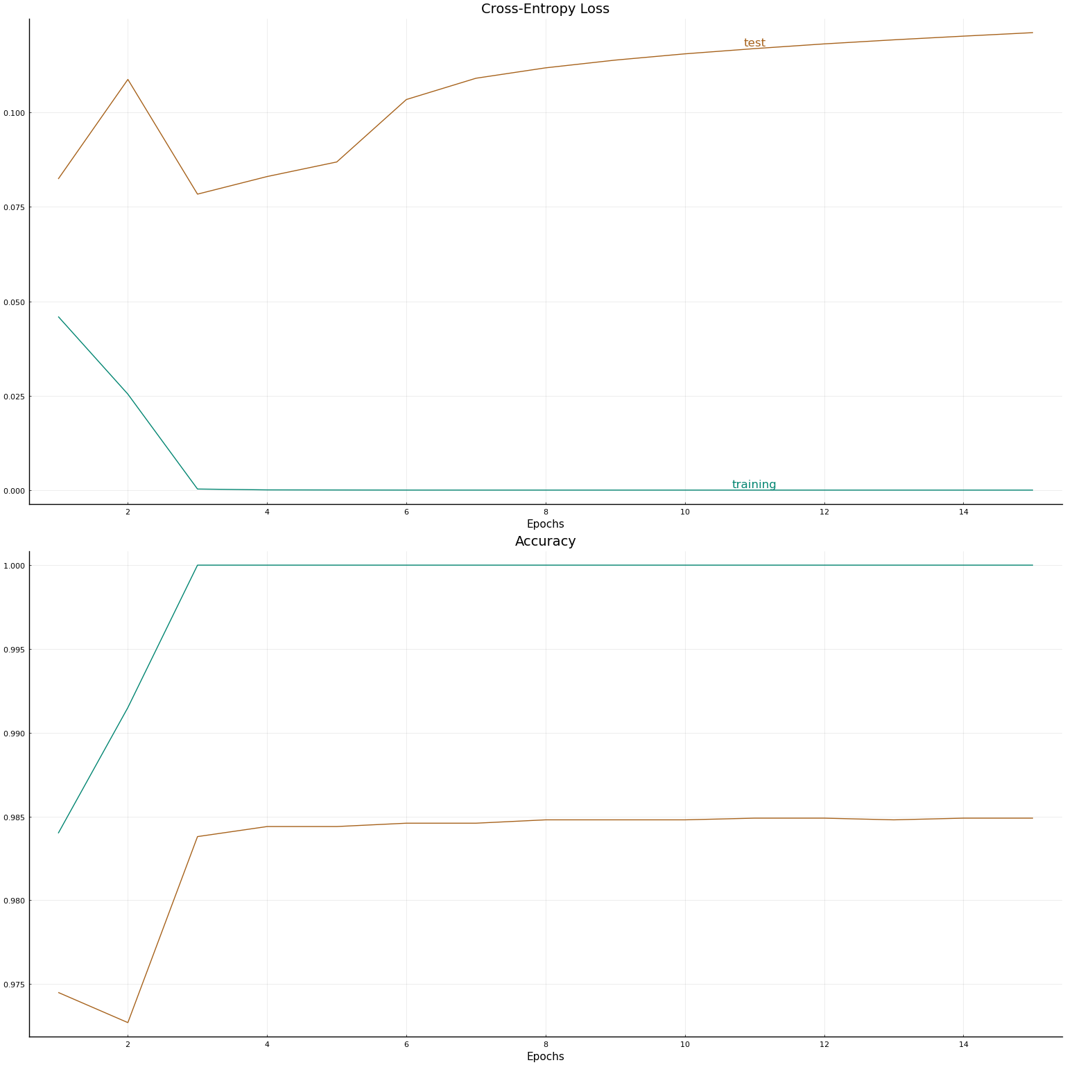
There is really something remarkable going on in this example. A model that appears extremely overparameterized manages to predict very well on a test set.

One important thing to keep in mind is that image classification is very different from the typical estimation problems in applied economics. In regressions and other models of economic variables, we never expect to be able to predict perfectly. An $R^2$ of 0.4 in a cross-sectional earnings regression is typical, or even high. Image classification is very different. We know there is a model (our eyes) that can classify nearly perfectly. In the language of econometrics, the error term is zero, or there is no uncertainty, in the “true” image classification models.

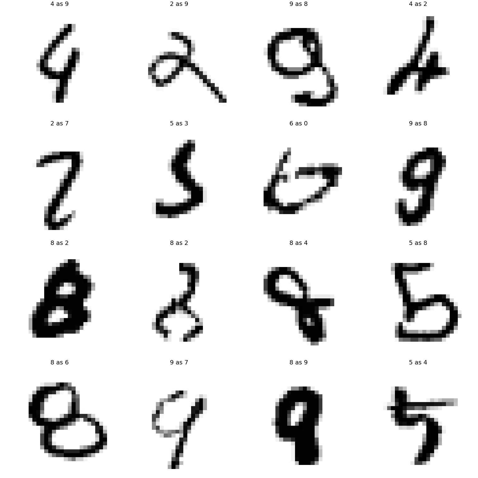
Let’s look at some of the images that our model failed to classify correctly.

timgs = [Gray.(1 .-test_x[:,:,i]') for i ∈ 1:size(test_x,3)]
tlabels = test_y

# predicted labels
mlabels = cpu(vec(map(x->x[1], argmax(cmgsnet(tX), dims=1)))) .- 1
@show mean(mlabels.==tlabels) # = accuracy
@show sum(mlabels .!= tlabels)
miss=findall(mlabels .!= tlabels)
plot( [plot(timgs[i], axis=false, ticks=false, title="$(tlabels[i]) as $(mlabels[i])", aspect_ratio=:equal) for i in miss[1:16]]...)

mean(mlabels .== tlabels) = 0.9842
sum(mlabels .!= tlabels) = 158

Our model still does not have state-of-the-art accuracy. (Ciresan et al. 2010)⁴ achieves 99.65% accuracy. There are differences in terms of activation function and gradient descent details between (Ciresan et al. 2010)⁴ and the code above. However, I suspect that the main reason for their better performance is that (Ciresan et al. 2010)⁴ generate additional training images. They do this by randomly rotating, stretching, and adding oscillations to the existing images.

Data Augmentation¶

Generating more data from your existing data is called data augmentation. Let’s try augmenting the data by randomly rotating the images.

function rotateimage(img, θ)
  R = similar(img)
  R .= img[1,1]
  i0 = (size(img,1)+1)/2
  j0 = (size(img,2)+1)/2
  for i ∈ axes(img)[1]
    for j ∈ axes(img)[2]
      ri = Int(round((i-i0)*cos(θ) + (j-j0)*sin(θ) +i0))
      rj = Int(round(-(i-i0)*sin(θ) + (j-j0)*cos(θ) +j0))
      if (ri ∈ axes(img)[1] && rj ∈ axes(img)[2])
        R[ri,rj] = img[i,j]
      end
    end
  end
  return R
end

plot([plot(timgs[i], axis=false, ticks=false, aspect_ratio=:equal) for i in 1:8]...,
    [plot(rotateimage(timgs[i], (-1)^i*π/6), axis=false, ticks=false, aspect_ratio=:equal) for i in 1:8]...)

Training with rotated images.

rerun = false
batchsize=10000
parts=Base.Iterators.partition(1:size(X,2), batchsize)
randrotate(x::AbstractVector; maxθ = π/8) = vec(rotateimage(reshape(x, 28, 28), rand()*2maxθ - maxθ))
data = [(gpu(mapslices(randrotate,cpu(X[:,p]), dims=1)), Y[:,p]) for p in parts for i=1:10];

epochs = 10
acctest  = zeros(epochs)
acctrain = zeros(epochs)
losstest  = zeros(epochs)
losstrain = zeros(epochs)
cmgsnet = gpu(cmgsnet_cpu)
opt=Flux.setup(ADAM(),cmgsnet)
for e in 1:epochs
  local modelfile = joinpath(modeldir,"cmgsnet-aug-$e-epochs.jld2")
  if rerun || !isfile(modelfile)
      println("Beginning epoch $e")
      evalcb(cmgsnet)
      @time Flux.train!(loss,
                        cmgsnet, data, opt)
      evalcb(cmgsnet)

      # save model
      local cpum = cpu(cmgsnet)
      modelstate = Flux.state(cpum)
      JLD2.@save modelfile modelstate
  else
      cpum = cpu(cmgsnet)
      JLD2.@load modelfile modelstate
      Flux.loadmodel!(cpum, modelstate)
      global cmgsnet = gpu(cpum)
  end
  println("Finished $e epochs")
  losstrain[e]=loss(cmgsnet,X,Y)
  acctrain[e]=accuracy(cmgsnet,Xsmall, Ysmall)
  losstest[e]=loss(cmgsnet,tX,tY)
  acctest[e]=accuracy(cmgsnet,tX,tY)
end
e = epochs
modelfile = joinpath(modeldir,"cmgsnet-aug-$e-epochs.jld2")
JLD2.@load modelfile modelstate
Flux.loadmodel!(cmgsnet, modelstate)

@show maximum(acctest)

Finished 1 epochs
Finished 2 epochs
Finished 3 epochs
Finished 4 epochs
Finished 5 epochs
Finished 6 epochs
Finished 7 epochs
Finished 8 epochs
Finished 9 epochs
Finished 10 epochs
maximum(acctest) = 0.9878
0.9878

timgs = [Gray.(1 .-test_x[:,:,i]') for i ∈ 1:size(test_x,3)]
tlabels = test_y

# predicted labels
mlabels = cpu(vec(map(x->x[1], argmax(cmgsnet(tX), dims=1)))) .- 1
@show mean(mlabels.==tlabels) # = accuracy
@show sum(mlabels .!= tlabels)
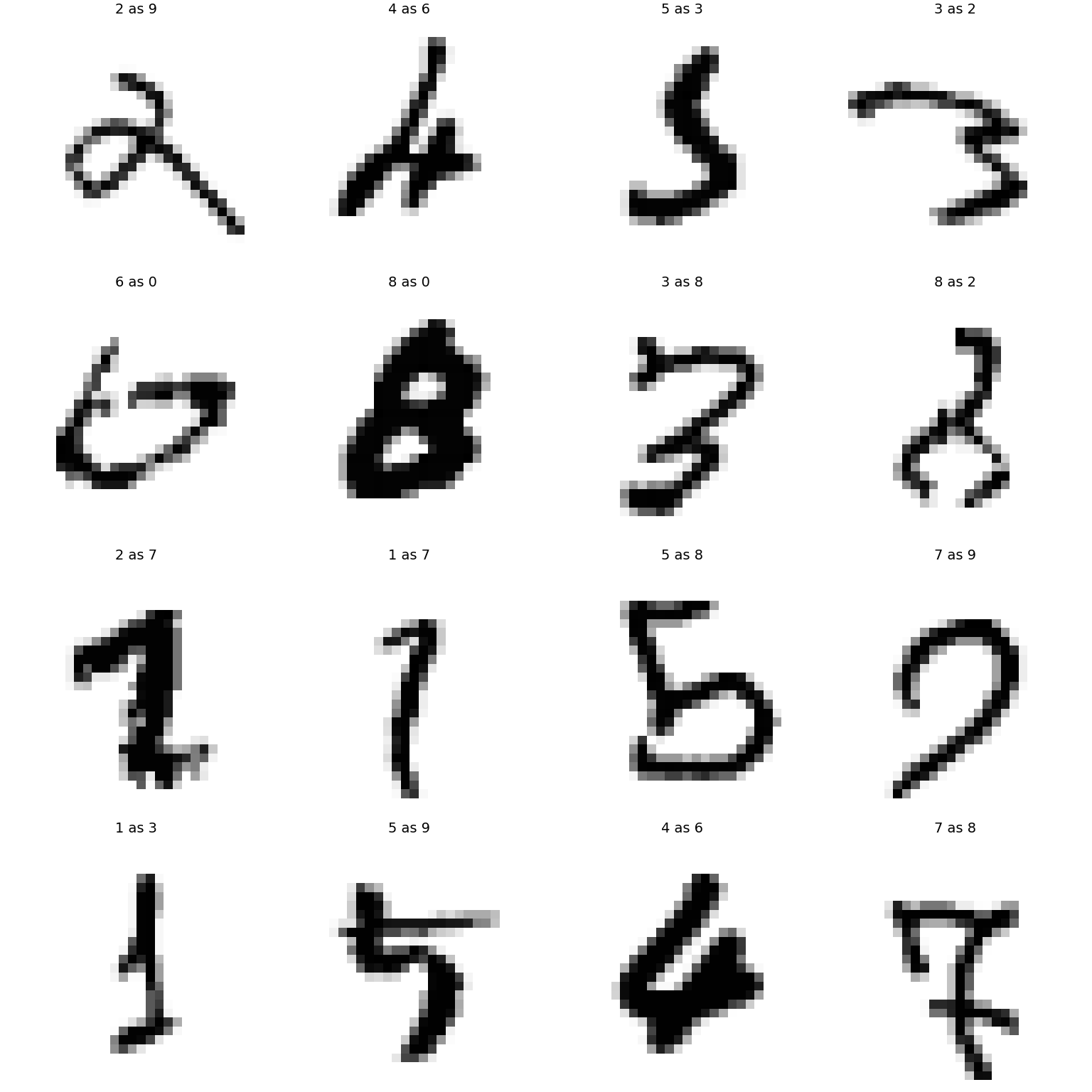
miss=findall(mlabels .!= tlabels)
plot( [plot(timgs[i], axis=false, ticks=false, title="$(tlabels[i]) as $(mlabels[i])", aspect_ratio=:equal) for i in miss[1:16]]...)

mean(mlabels .== tlabels) = 0.9858
sum(mlabels .!= tlabels) = 142

References¶

Goodfellow, Ian, Yoshua Bengio, and Aaron Courville, “Deep learning,” (MIT Press, 2016). ↩
Klok, Hayden, and Yoni Nazarathy, “Statistics with julia:fundamentals for data science, MachineLearning and artificial intelligence,” (DRAFT, 2019). ↩
Farrell, Max H., Tengyuan Liang, and Sanjog Misra, “Deep neural networks for estimation and inference,” 2018. ↩↩
Ciresan, Dan Claudiu, Ueli Meier, Luca Maria Gambardella, and Juergen Schmidhuber, “Deep big simple neural nets excel on handwritten digit recognition,” 2010 (Neural Computation, Volume 22, Number 12, December 2010). ↩↩↩↩

Keys	Action
`?`	Open this help
`n`	Next page
`p`	Previous page
`s`	Search