This work is licensed under a Creative Commons Attribution-ShareAlike 4.0 International License

About this document¶

This document was created using Weave.jl. The code is available in on github. The same document generates both static webpages and associated jupyter notebook.

$$\def\indep{\perp\!\!\!\perp} \def\Er{\mathrm{E}} \def\R{\mathbb{R}} \def\En{{\mathbb{E}_n}} \def\Pr{\mathrm{P}} \newcommand{\norm}[1]{\left\Vert {#1} \right\Vert} \newcommand{\abs}[1]{\left\vert {#1} \right\vert} \DeclareMathOperator*{\argmax}{arg\,max} \DeclareMathOperator*{\argmin}{arg\,min}$$

Introduction¶

We have now covered a variety of neural network architectures and seen examples of how they are used for classic machine learning tasks. How can neural networks be incorporated into typical economic research?

There are two important differences between empirical economics and the digit classification and text generation examples we looked at:

1. Economic data has a lot more inherent uncertainty. In both images and text, we know there is a nearly perfect model (our eyes and brain). In economics, perfect prediction is almost never possible. For example, if we could predict stock prices even slightly more accurately than a random walk, then we could be billionares.

2. In part related to 1, economists care about statistical inference and quantifying uncertainty.

Both of these factors are going to make concerns about overfitting and model complexity more important.

This note will focus on one way to use neural networks in estimable economic models that allows inference. Inference directly on the nonparametric function fitted by a neural network is a very difficult problem. There are practical methods for Bayesian variational inference (see (Graves 2011)² or (Miao, Yu, and Blunsom 2016)³), but frequentist inference is largely an open problem.

However, what is possible is semiparametric inference. Semiparametric inference refers to when we have a finite dimensional parameter of interest that depends on some infinite dimensional parameter. Examples include average (or quantiles or other summary statistic) marginal effects, average treatment effects, and many others.

Double Debiased Machine Learning¶

We return to the semiparametric moment condition model of (Chernozhukov et al. 2018)⁴ and (Chernozhukov et al. 2017)⁵. We previously discussed this setting in ml-intro and ml-doubledebiased.

The model consists of

• Parameter of interest $\theta \in \R^{d_\theta}$

• Nuisance parameter $\eta \in T$ (where $T$ is typically some space of functions)

• Moment conditions $$\Er[\psi(W;\theta_0,\eta_0) ] = 0 \in \R^{d_\theta}$$ where $\psi$ known

See ml-intro and ml-doubledebiased for examples.

The estimation procedure will proceed in two steps:

1. Estimate $\hat{\eta}$ from a neural network

2. Estimate $\hat{\theta}$ from the empirical moment condition with $\hat{\eta}$ plugged in: $$\En[\psi(W;\hat{\theta},\hat{\eta}) ] \approx 0$$

(Chernozhukov et al. 2018)⁴ provide high level assumptions on $\hat{\eta}$ and the model that ensure $\hat{\theta}$ is $\sqrt{n}$ asymptotically normal.¹ The key needed assumptions are:

1. Linearizeable score $$\psi(w;\theta,\eta) = \psi^a(w;\eta) \theta + \psi^b(w;\eta) + o_p(?)$$
2. (Near) Neyman orthogonality: $$\lambda_n := \sup_{\eta \in \mathcal{T}_n} \norm{\partial \eta \Er\left[\psi(W;\theta_0,\eta_0)[\eta-\eta_0] \right] } \leq \delta_n n^{-1/2}$$
3. Fast enough convergence of $\hat{eta}$: for $\delta_n \to 0$ and $\Delta_n \to 0$, we have $\Pr(\hat{\eta}_k \in \mathcal{T}_n) \geq 1-\Delta_n$ and $$\begin{align*} r_n := & \sup_{\eta \in \mathcal{T}_n} \norm{ \Er[\psi^a(W;\eta)] - \Er[\psi^a(W;\eta_0)]} \leq \delta_n \\ r_n' := & \sup_{\eta \in \mathcal{T}_n} \Er\left[ \norm{ \psi(W;\theta_0,\eta) - \psi(W;\theta_0,\eta_0)}^2 \right]^{1/2} \leq \delta_n \\ \lambda_n' := & \sup_{r \in (0,1), \eta \in \mathcal{T}_n} \norm{ \partial_r^2 \Er\left[\psi(W;\theta_0, \eta_0 + r(\eta - \eta_0)) \right]} \leq \delta_n/\sqrt{n} \end{align*}$$

Assumption 1 is stated here mostly to define notation 3. A model where $\psi$ is not linearizeable would be unusual.

Assumption 2 must be satisfied by each application. In many models, the most obvious choice of $\psi$ will not satisfy 2. However, $\psi$ can be orthogonalized to satisfy 2.

Assumption 3 is about the convergence rate of our estimator for $\hat{\eta}$. It is written this way because it exactly what is needed for the proof; it is not intended to be easy to interpret or to verify. A sufficient, but not necessary condition that implies 3 is twice differentiability of $\psi$ and $\Er[(\hat{\eta}(x) - \eta_0(x))^2]^{1/2} = o(n^{-1/4})$.

Anyway, (Chernozhukov et al. 2018)⁴ show that under these conditions (and if you use sample splitting in the empirical moment condition), then $$\sqrt{n} \sigma^{-1} (\hat{\theta} - \theta_0) = \frac{1}{\sqrt{n}} \sum_{i=1}^n \bar{\psi}(w_i) + O_p(\rho_n) \leadsto N(0,I)$$ where $$\rho_n := n^{-1/2} + r_n + r_n' + n^{1/2} (\lambda_n +\lambda_n') \lesssim \delta_n$$ and $\bar{\psi}$ is the influence function, $$\bar{\psi}(w) = -\sigma^{-1} J_0^{-1} \psi(w;\theta_0,\eta_0)$$ with $$\sigma^2 = J_0^{-1} \Er\left[ \psi(w;\theta_0,\eta_0) \psi(w;\theta_0,\eta_0)'\right] (J_0^{-1})'.$$ This is the same asymptotic distribution as if we plugged in the true $\eta_0$ instead of our estimated $\hat{\eta}$.

To apply this result to neural networks we need two things. First, we need to verify the rate condition (assumption 2). Doing so will involve conditions on the class of functions being estimated, and how the complexity (width and depth) of the neural network increases with sample size. The excellent paper by (Farrell, Liang, and Misra 2021)⁶ (working paper (Farrell, Liang, and Misra 2018)⁷) provides the needed results.

Second, we need to make sure our moment conditions are Neyman orthogonal. (Chernozhukov et al. 2018)⁴ and (Farrell, Liang, and Misra 2021)⁶ do this for some typical causal inference models. For other models, analytically transforming non-orthogonal moments into orthogonal ones is typically possible, but it can be tedious.

Deep Neural Networks for Estimation and Inference¶

Review results of (Farrell, Liang, and Misra 2021)⁶.

Application: Average Impulse Responses¶

As an application let’s consider something like an average impulse response function. Suppose we have some time series data on $y_t$ and $x_t$. We want to estimate the average (over the density of $x$) response of $\Er[y_{t+\tau} | x_t]$ to a change in $x$ of size $\Delta$. That is, our parameters of interest are $$\theta_{0,\tau} = \Er\left[ \Er[y_{t+\tau} | x_{t} + \Delta] - \Er[y_{t+\tau} | x_{t}] \right]$$ for $\tau = 0, …, R$ for some fixed $R$.

::: {.alert .alert-danger} Note that there are other impulse response like parameters that could be estimated. For example, we could compute the average over $x_t$ of the change in future $y$ holding future residuals constant (or setting future residuals to $0$). In a linear model this would be the same as the average over residuals response that we estimate. However, in a nonlinear model, these three things differ. We focus on the average over residuals response in part because orthogonalization of the moment condition is more difficult for the later two. :::

Let $h(x_t) = (\Er[y_{t} | x_{t}], … , \Er[y_{t+R} | x_{t}])$ denote the conditional expectation functions at different horizons. Then, we can write a moment condition for $\theta_0$ as: $$0 = \Er[ \theta_0 - \left(h(x_t + \Delta) - h(x_t) \right)].$$ However, this moment condition is not orthogonal. Its Frechet derivative with respect to $h$ in direction $v$ is $$\partial_h\left(\Er[ \theta - \left(h_0(x_t + \Delta) - h(x_t) \right)] \right) [v] = \Er[-v(x_t + \Delta) + v(x_t)] \neq 0.$$

We can orthogonalize the moment condition by following the concentrating out approach described in (Chernozhukov et al. 2018)⁴, or in ml-doubledebiased. It would be a good exercise to work through the steps. Here we will simply state a resulting orthogonal moment condition. Let $\eta=(h, f_x)$ where $f_x$ is the density of $x$. Define $$\psi(y,x;\theta, \eta) = \theta - (h(x+\Delta) - h(x))) + (y - h(x))\frac{-f_x(x-\Delta)+f_x(x)} {f_x(x)}$$

Although somewhat difficult to derive, it is easy to verify that $\Er \psi$ is orthogonal. $$\begin{align*} \partial_h \left(\Er[ \psi(y_t,x_t;\theta_0, \eta_0) ] \right) [v] = & \Er\left[-v(x_t + \Delta) + v(x_t) + v(x_t +\Delta) - v(x_t)\right] = 0 \\ \partial_{f_x} \left(\Er[ \psi(y_t,x_t;\theta_0, \eta_0) ] \right) [v] = & \Er\left[(E[y|x] - h_0(x)) \frac{(-v(x+\Delta) + v(x))f_x(x) - v(x)}{f_x(x)^2} \right] = 0 \end{align*}$$ Notice that to achieve orthogonality, we had to introduce an additional functional nuisance parameter, $f_x$. This is typical in these models.

Simulated DGP¶

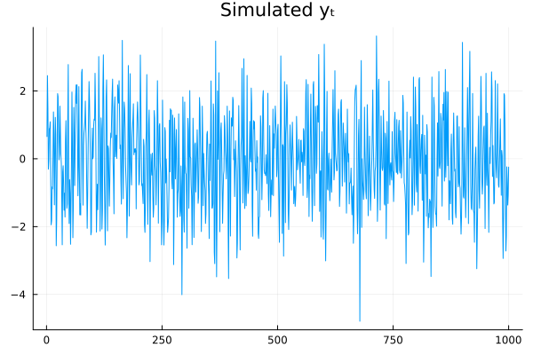
Let’s do some simulations to examine the performance of this estimator. The true model will be a nonlinear AR(3) model. In particular, $$y_t = \tanh(\alpha_1 y_{t-1} + \alpha_2 y_{t-2} + \alpha_3 y_{t-3}) + \epsilon_t$$

using Polynomials, Plots, LinearAlgebra, Statistics, Random
Random.seed!(747697)
T = 1000
R = 50
θ = 0.1
r = 0.99

# We start with an AR(P). We specify coefficients by choosing the
# roots of the AR polynomial.  In a linear model, complex roots on the
# unit circle lead to non-vanishing cycles in y.
roots = [r*exp(im*θ),   r*exp(-im*θ), 0.5]

p = prod([Polynomial([1, -r]) for r in roots])
α = -real(coeffs(p))[2:end]
function mean_y_fn(α, transform=(x)->x)
  ylag->transform(dot(ylag, α))
end
function dgp(mean_y, T, sig=1, yinit=zeros(length(α)))
  ylag = yinit
  y = zeros(T)
  for t in 1:T
    y[t] = muladd(sig, randn(),mean_y(ylag) )
    ylag[2:end] .= ylag[1:(end-1)]
    ylag[1] = y[t]
  end
  return(y)
end

μy = mean_y_fn(α, x->1/r*tanh(x))
y = dgp(μy, T, 1.0)
plot(y, title="Simulated yₜ", leg=false)

R = 12
L = length(α)
Δ = 1.0*std(y)
nsim = 1000
iry=reduce(hcat,[mean(x->(dgp(μy , R, 1.0, y[i:(i+L-1)] .+ [Δ, 0, 0]) .-
                          dgp(μy , R, 1.0, y[i:(i+L-1)]) ),  1:nsim)
                 for i in 1:(T-length(α)+1)])./std(y)
plot(iry, leg=false, alpha=0.01, color=:black, linewidth=1)
plot!(mean(iry, dims=2), leg=false, linewidth=5, title="E[Δy | 1σ change in y]",
      xlab="τ", ylab="ΔE[y(t+τ)]/std(y)", alpha=1)

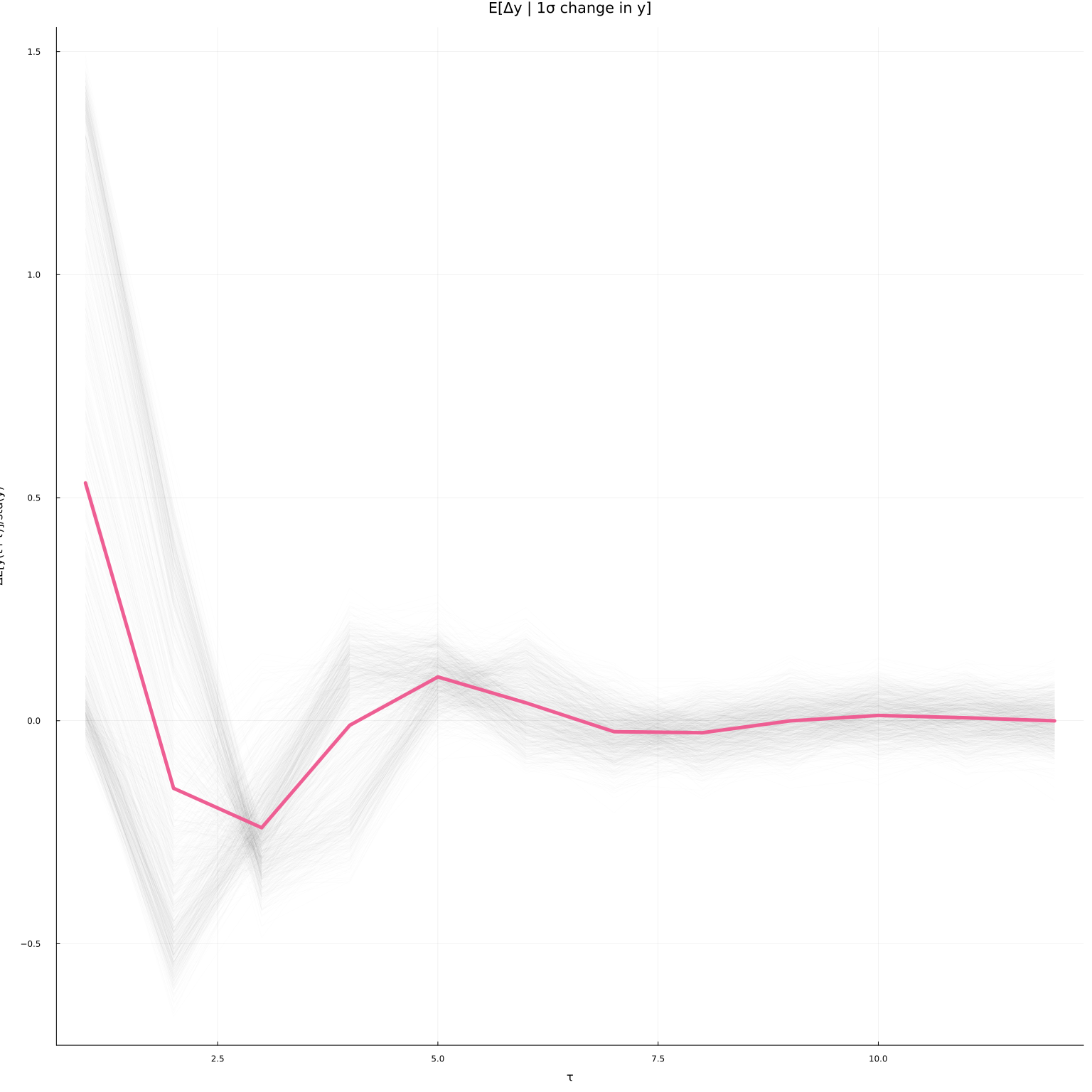
The conditional average impulse responses at each $x_t=(y_{t-1}, …, y_{t-p})$ in the simulated data are in grey. The average over $x_t$ is the thicker green-ish line. In a linear model the average and conditional impulse responses coincide. In this model, they differ because of the nonlinearity.

Estimators¶

To somewhat simplify this exercise, we will assume that the researcher knows that $y$ follows a nonlinear AR(3) model. That is, we know that $$y_t = h(y_{t-1}, y_{t-2}, y_{t-3}) + \epsilon_t$$ We will estimate $h$ using this knowledge. To estimate the impulse response, we need estimates of the conditional expectation of $y$ and the density of $x_t = (y_{t-1}, y_{t-2}, y_{t-3})$.

Density¶

We will estimate the density as the derivative of a feed forward network. We fit the a feed forward network to the empirical cdf. We penalize the estimated cdf for not being monotone. Here is code to fit the model.

using Flux, ProgressMeter, JLD2
using CUDA
import Base.Iterators: partition
L = length(α)
x = copy(reduce(hcat,[y[l:(end-L+l)] for l in L:-1:1])')

function fit_cdf!(model, x;
                  opt=Flux.setup(Flux.NADAM(),model),
                  maxiter=1000, λ = eltype(x)(1.0), n_extra=0,
                  batchsize=length(x) + n_extra)
    # we could augment cdf evaluation points with x not seen in the data
    # in 1-d, there is no need, but in multiple dimension, there's extra info.
    i = 0
    X = x
    if (n_extra>0)
        CUDA.@allowscalar X=hcat(x, rand(x, size(x,1), n_extra))
    end
    CUDA.@allowscalar ecdf = eltype(x).(mapslices( xi->mean(all(X .<= xi, dims=1)), X, dims=1 ))
    Δ = gpu(diagm(fill(eltype(x)(0.01), size(x,1))))

    monotone_penalty = if λ > 0
        (model,x,cdf) -> λ*sum(δ->sum( relu.(model(x) .- model(x .+ δ))), eachcol(Δ))
    else
        (model,x,cdf) -> zero(eltype(x))
    end
    loss(model,x,cdf) = Flux.mse(model(x), cdf) + monotone_penalty(model,x, cdf)
    @show bestloss = loss(model,X,ecdf)+1
    lastimprove=0
    p = Progress(maxiter, 1)
    data = [(X[:,p], ecdf[:,p]) for p in partition(1:size(X,2), batchsize)]
    for i in 1:maxiter
        Flux.train!(loss, model,
                    data, opt)
        obj = loss(model,X, ecdf)
        next!(p)
        (i%(maxiter ÷ 10) == 0) && println("\n$i : $obj")
        if (obj < bestloss)
            bestloss=obj
            lastimprove=i
        end
        if (i - lastimprove > 300)
            println("\n$i : $obj")
            @show lastimprove, bestloss
            @warn "no improvement for 300 iterations, stopping"
            break
        end
    end
    return(model)
end

fit_cdf! (generic function with 1 method)

We can recover the pdf from the cdf by differentiating. For univariate distributions, this is easy. However, for multivariate distributions, $$f_x(x) = \frac{\partial^n}{\partial x_1 \partial x_2\cdots \partial x_n} F_x(x)$$ so we need to evaluate an $n$th order derivative. Here is some code to do so.

using ForwardDiff
function deriv_i(f, i)
  # derivative wrt to ith argument
  dfi(z)=ForwardDiff.derivative((y)->f([z[1:(i-1)]..., y, z[(i+1):end]...]), z[i])
end

function make_pdf(cdf, dim)
  fs = Function[]
  push!(fs, x->cdf(x))
  for i in 1:dim
    push!(fs, deriv_i(fs[end], i))
  end
  function f(x::AbstractVector)
    fs[end](x)
  end
  function f(x::AbstractMatrix)
    mapslices(fs[end], x, dims=1)
  end
  return(f)
end

make_pdf (generic function with 1 method)

To check that the code produces reasonable results, we will begin by just fitting the marginal distribution of $y_t$. This isn’t quite what we need for our impulse responses, but it is easier to visualize.

modelfile=joinpath(docdir,"jmd","models","cdfy.jld2")
rerun=false
cdfy = Chain(
    Dense(1, 100, Flux.σ),
    Dense(100, 100, Flux.σ),
    Dense(100, 100, Flux.σ),
    Dense(100, 100, Flux.σ),
    Dense(100, 1, Flux.σ)
)
if isfile(modelfile) && !rerun
    JLD2.@load modelfile modelstate
    Flux.loadmodel!(cdfy, modelstate)
else
    cdf_model = gpu(cdfy)
    fit_cdf!(cdf_model, gpu(reshape(Float32.(y), 1, T)),
             maxiter=10000, λ=1e4 )
    cdfy = cpu(cdf_model)
    modelstate = Flux.state(cdfy)
    JLD2.@save modelfile modelstate
end
pdfy = make_pdf(cdfy, 1)

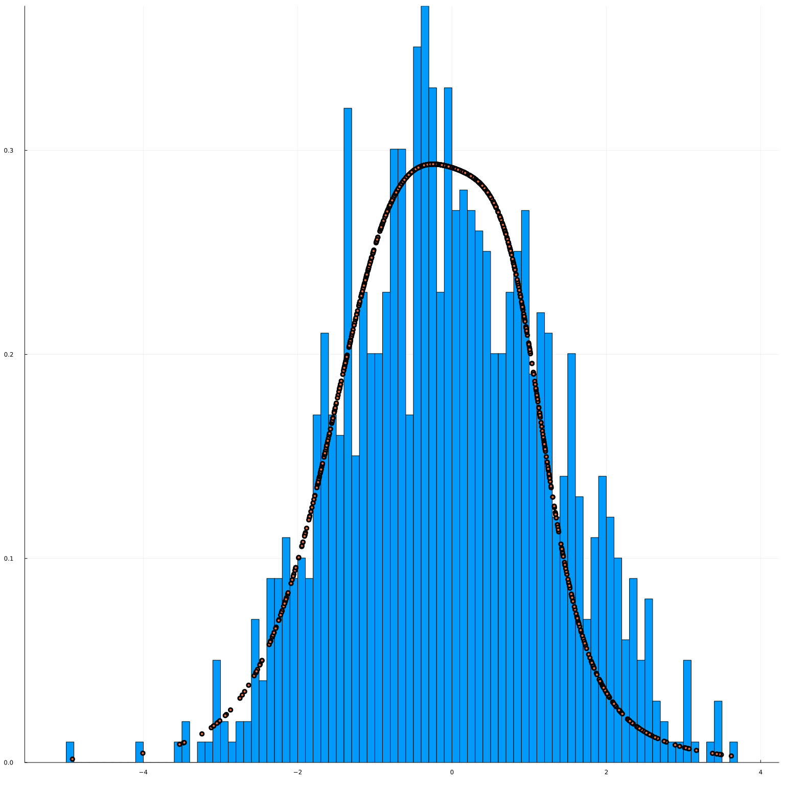
fig=histogram(y, bins=100, normalize=:pdf)
fig=scatter!(y, pdfy(reshape(y,1,T))[:], leg=false)

The estimated pdf looks pretty good.

We will estimate the joint cdf and pdf similarly.

modelfile=joinpath(docdir,"jmd","models","cdfx.jld2")
K = 100
cdfx =  Chain(
    Dense(3, K, Flux.σ),
    Dense(K, K, Flux.σ),
    Dense(K, K, Flux.σ),
    Dense(K, K, Flux.σ),
    Dense(K, 1, Flux.σ)
  )
if isfile(modelfile) && !rerun
    JLD2.@load modelfile modelstate
    Flux.loadmodel!(cdfx, modelstate)
else
    cdf_model = gpu(cdfx)
    @time fit_cdf!(cdf_model, gpu(Float32.(x)), opt=Flux.setup(NADAM(),cdf_model),
                   maxiter=10000, λ=0, n_extra=20_000)
    cdfx = cpu(cdf_model)
    modelstate = Flux.state(cdfx)
    JLD2.@save modelfile modelstate
end
pdfx = make_pdf(cdfx, size(x,1))
@show sum(pdfx(x).<0)
histogram(pdfx(x)', bins=100, leg=false, title="Histogram of estimated pdf(x)")

sum(pdfx(x) .< 0) = 40

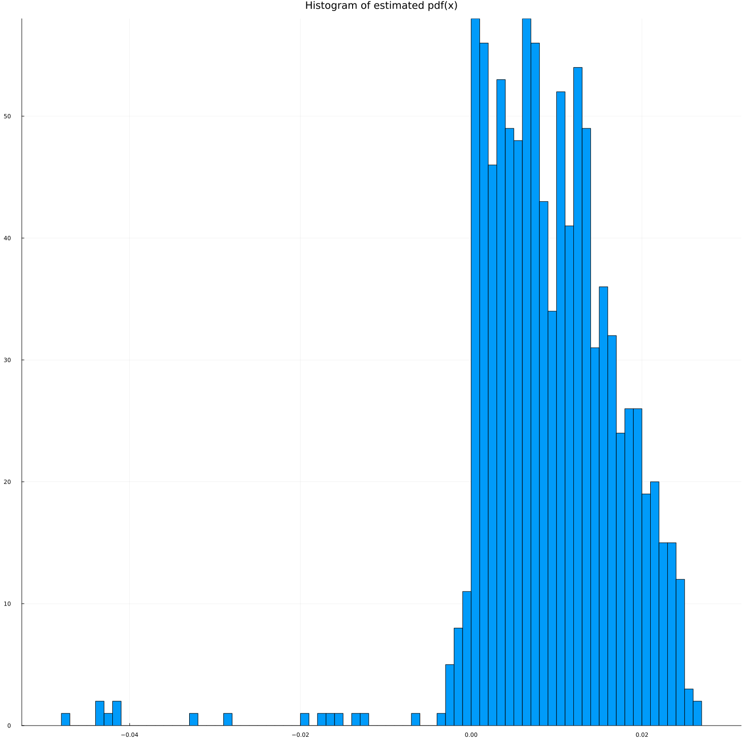
Despite the penalty, our estimated pdf is sometimes negative. Fortunately, it doesn’t happen to often.

It’s hard to visualize the estimated trivariate pdf, but we can plot the marginal pdf implied by the joint distribution. We can get marginal pdf by integrating or looking at the derivative of the joint cdf. $$f_{x_1}(x_1) = \frac{\partial}{\partial x_1} F_x((x_1, \overline{x}_2, \overline{x}_3))$$ where $\overline{x}_k$ is the maximum of the support of $x_k$.

pdf12=make_pdf(cdfx,2)
pdf1=make_pdf(cdfx,1)
px1=pdf1(vcat(x[1,:]', maximum(y)*ones(2, 998)))
histogram(x[1,:], bins=100, normalize=:pdf)
scatter!(x[1,:], px1[:], leg=false)

The marginal pdf implied by the joint cdf looks okay.

Note, however, that to get this result, I had to specify a fairly complex network, which took around a minute to fit. There are many other ways to estimate densities, and another approach might have made more sense here.

Conditional expectation¶

We will assume that we that knows that $y$ follows a nonlinear AR(3) model. Then, we can simply fit a feed forward network to predict $y_t$ given $x_t = (y_{t-1}, y_{t-2}, y_{t-3})$.

function fit_ce!(model, x, y;
                 opt=Flux.setup(Flux.NADAM(),model), maxiter=1000, batchsize=length(y))
  loss(model,x,y) = Flux.mse(model(x), y)
  @show bestloss = loss(model,x,y)+1
  lastimprove=0
  p = Progress(maxiter, 1)
  data = [(x[:,p], y[:,p]) for p in partition(1:size(x,2), batchsize)]
  for i in 1:maxiter
    Flux.train!(loss, model,
                data, opt)
    obj = loss(model,x,y)
    next!(p)
    (i%(maxiter ÷ 10) == 0) && println("\n$i : $obj")
    if (obj < bestloss)
      bestloss=obj
      lastimprove=i
    end
    if (i - lastimprove > 300)
      @warn "no improvement for 300 iterations, stopping"
      break
    end
  end
  return(model)
end

R = 12 # how many periods ahead to fit
Y = copy(reduce(hcat,[y[(L+r):(end-R+r)] for r in 1:R])')
X = x[:,1:(end-R)]

modelfile=joinpath(docdir,"jmd","models","ce.jld2")
K = 100
ce_model = Chain(Dense(size(X,1), K, relu),
                 Dense(K, K, relu),
                 Dense(K, K, relu),
                 Dense(K, size(Y,1))) |> gpu
if !isfile(modelfile) || rerun
    fit_ce!(ce_model, gpu(Float32.(X)), gpu(Float32.(Y)),
            opt=Flux.setup(Flux.NADAM(),ce_model),
            maxiter=20000, batchsize=size(Y,2))
    cpum = cpu(ce_model)
    modelstate = Flux.state(cpum)
    JLD2.@save modelfile modelstate
end
cpum = cpu(ce_model)
JLD2.@load modelfile modelstate
Flux.loadmodel!(cpum, modelstate)
ce_model = gpu(cpum)

μhat(x) = let m=cpu(ce_model)
  m(x)
end
μhat(x::AbstractVector) = let m=cpu(ce_model)
  eltype(x)(m(x)[1])
end

μhat (generic function with 2 methods)

Finally, we can calculate the orthogonalized impulse responses. As stated above, these are given by $$\theta = (h(x+\Delta) - h(x))) + (y - h(x))\frac{-f_x(x-\Delta)+f_x(x)} {f_x(x)}$$

Let’s compute it

L = size(x,1)
Δ = 1.0*std(y)
iryhat=(μhat(X .+ [Δ; 0; 0])  .- μhat(X))
fx(x) = max.(pdfx(x), 1e-3)
ℓ(x) = (fx(X) .- fx(X .- [Δ; 0; 0]))./fx(X)
lx = ℓ(x)[:]
c = quantile(lx, [0.02, 0.98])
idx = Int.(findall((c[1] .<= lx) .& (lx .<= c[2])))
θi = μhat(X .+ [Δ; 0; 0])  .- μhat(X) .+ (Y .- μhat(X)).*ℓ(X)
#θi = θi[:,idx]

12×986 Matrix{Float64}:
  2.74115      0.633616   1.46919   …   2.83516    0.478738   0.988624
  1.52376     -2.19382   -0.600689      3.51889   -0.302066  -0.893764
  0.0877915   -0.211538  -3.7528        2.603      0.428047  -1.33342
  0.266089     3.87247   -0.863443     -0.450994  -1.50694    0.150621
  0.462978     1.51076    5.24261      -2.05753   -0.915333   0.864609
 -0.416113    -1.19463    6.91263   …  -2.00228    2.5386     1.88317
  0.00347961   3.16738    0.456882      1.28134    1.34017    1.98044
  2.39451      1.82583    1.12062       3.34856   -1.61011    1.18015
  1.80234      0.893354   0.42969       1.95434   -0.98422    1.83293
 -1.17812      1.89823   -4.03694       1.86311   -0.418697   2.76707
 -1.16722      3.79379   -0.676402  …   1.66644   -0.392824   0.707905
  0.280006     0.866211   8.30275       1.20111    0.837611  -0.926341

and plot it

#plot(iry, leg=false, alpha=0.02, color=:black, linewidth=1)
#plot!(iryhat, leg=false, alpha=0.02, color=:orange, linewidth=1, ylim=(-0.5, 0.75))
#plot!(θi, leg=false, alpha=0.01, color=:green, linewidth=1, ylim=(-0.5, 0.75))
plot(mean(iry, dims=2), leg=false, linewidth=5, title="Average Impulse-Reponse to 1σ change in y[t-1]",
     xlab="τ", ylab="ΔE[y(t+τ)]/std(y)", color=:blue)
plot!(mean(iryhat, dims=2), leg=false, linewidth=5, color=:orange)
plot!(mean(θi, dims=2), leg=false, linewidth=5, color=:green)

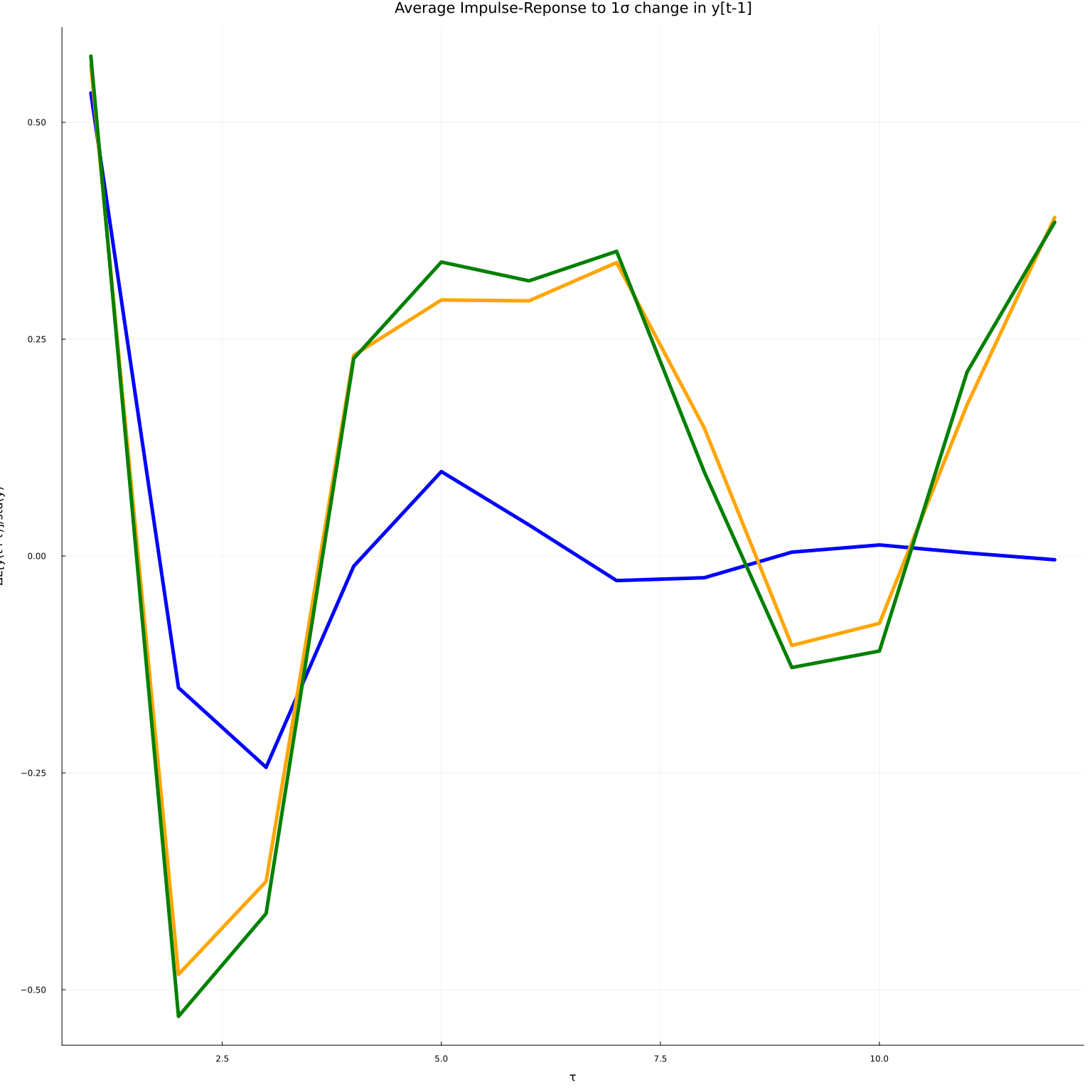
The true average impulse response is in blue. The uncorrected estimate is in orange. The orthogonalized estimate is in green.

Depending on the luck of RNG, and how well I have chosen the network architectures, the orthogonalized or naive point estimate might look better. However, the motivation is the orthogonalization is not so much to improve point estimation (although it does that as a side effect), but to enable inference.

Inference¶

Inference for the orthogonalized estimator is very simple. Due to the orthogonalization, we can treat μhat and fx as though they are known functions. The estimated average impulse response is then just a sample average. Computing standard errors for sample averages is straightforward.

using Distributions
using Statistics
Σ = cov(θi')

plot(iry, leg=false, alpha=0.02, color=:black, linewidth=1)
plot!(iryhat, leg=false, alpha=0.02, color=:orange, linewidth=1, ylim=(-0.5, 0.75))
#plot!(θi, leg=false, alpha=0.01, color=:green, linewidth=1, ylim=(-0.5, 0.75))
plot!(mean(iry, dims=2), leg=false, linewidth=5, title="Average Impulse-Reponse to 1σ change in y[t-1]",
     xlab="τ", ylab="ΔE[y(t+τ)]/std(y)", color=:blue)
plot!(mean(iryhat, dims=2), leg=false, linewidth=5, color=:orange)
plot!(mean(θi, dims=2), leg=false, linewidth=5, color=:green,
      ribbon=sqrt.(diag(Σ)/size(θi,2))*quantile.(Normal(), [0.05, 0.95])' )

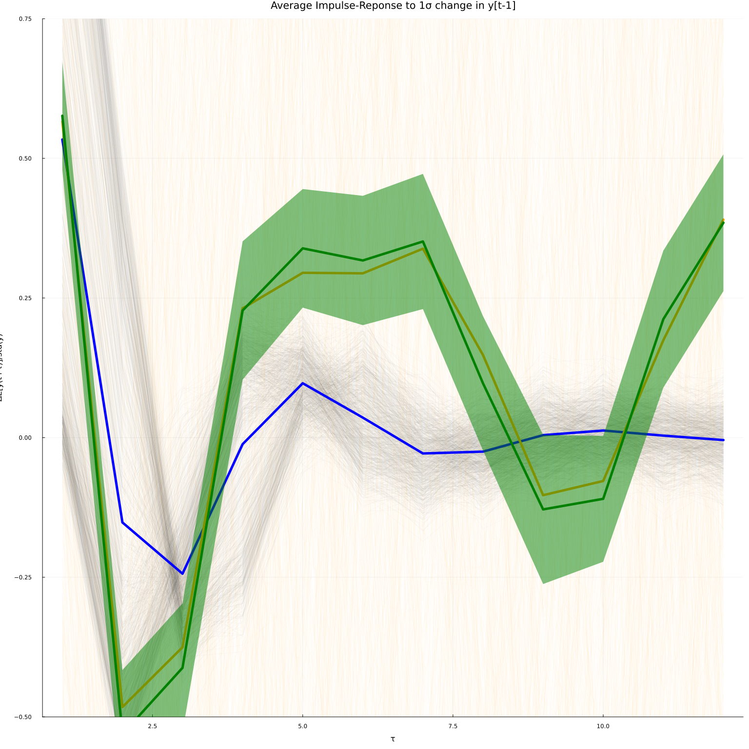
The plot now has 90% pointwise confidence bands around the orthogonalized estimates.

For an approach to debiased ML without analytically deriving orthogonal moment conditions, see the next section.