title : “Introduction to Neural Networks” subtitle : “Single Layer Perceptrons” author : Paul Schrimpf date : 2026-03-30 bibliography: “../ml.bib” weave_options: out_width : 100% wrap : true fig_width : 8 dpi : 192 —

This work is licensed under a Creative Commons Attribution-ShareAlike 4.0 International License

About this document¶

This document was created using Weave.jl. The code is available in on github. The same document generates both static webpages and associated jupyter notebook.

$$\def\indep{\perp\!\!\!\perp} \def\Er{\mathrm{E}} \def\R{\mathbb{R}} \def\En{{\mathbb{E}_n}} \def\Pr{\mathrm{P}} \newcommand{\norm}[1]{\left\Vert {#1} \right\Vert} \newcommand{\abs}[1]{\left\vert {#1} \right\vert} \DeclareMathOperator*{\argmax}{arg\,max} \DeclareMathOperator*{\argmin}{arg\,min}$$

Introduction¶

Neural networks, especially deep neural networks, have come to dominate some areas of machine learning. Neural networks are especially prominent in natural language processing, image classification, and reinforcement learning. This documents gives a brief introduction to neural networks.

Examples in this document will use Flux.jl. An alternative Julia package for deep learning is Knet.jl. There is a good discussion comparing Flux and Knet on discourse.. We will not have Knet examples here, but the documentation for Knet is excellent and worth reading even if you plan to use Flux.

Additional Reading¶

• (Goodfellow, Bengio, and Courville 2016)¹ Deep Learning
• Knet.jl documentation especially the textbook
• (Klok and Nazarathy 2019)² Statistics with Julia:Fundamentals for Data Science, MachineLearning and Artificial Intelligence

Single Layer Neural Networks¶

We will describe neural networks from a perspective of nonparametric estimation. Suppose we have a target function, $f: \R^p \to \R$. In many applications the target function will be a conditional expectation, $f(x) = \Er[y|x]$.

A single layer neural network approximates $f$ as follows $$\hat{f}(x) = \sum_{j=1}^r \beta_j \psi(w_j'x + b_j)$$ Here $r$ is the width of the layer. $\beta_j$ are scalars. $\psi:\R \to \R$ is a nonlinear activation function. Common activation functions include:

• Sigmoid $\psi(t) = 1/(1+e^{-t})$

• Tanh $\psi(t) = \frac{e^t -e^{-t}}{e^t + e^{-t}}$

• Rectified linear $\psi(t) = t 1(t\geq 0)$

The $w_j \in \R^p$ are called weights and $b_j \in \R$ are biases.

You may have heard about the universal approximation theorem. This refers to the fact that as $r$ increases, a neural network can approximate any function. Mathematically, for some large class of functions $\mathcal{F}$,

$$\sup_{f \in \mathcal{F}} \lim_{r \to \infty} \inf_{\beta, w, b} \Vert f(x) - \sum_{j=1}^r \beta_j \psi(w_j'x+b_j) \Vert = 0$$

(Hornik, Stinchcombe, and White 1989)³ contains one of the earliest results along these lines. Some introductory texts mention the universal approximation theorem as though it is something special for neural networks. This is incorrect. In particular, the universal approximation theorem does not explain why neural networks seem to be unusually good at prediction. Most nonparametric estimation methods (kernel, series, forests, etc) are universal approximators.

Training¶

Models in Flux.jl all involve a differentiable loss function. The loss function is minimized by a variant of gradient descent. Gradients are usually calculated using reverse automatic differentiation (backpropagation usually refers to a variant of reverse automatic differentiation specialized for the structue of neural networks).

Low level¶

A low level way to use Flux.jl is to write your loss function as a typical Julia function, as in the following code block.

using Plots, Flux, Statistics, ColorSchemes
# some function to estimate
_f(x) = sin(x^x)/2^((x^x-π/2)/π)
function simulate(n,σ=1)
  x = rand(n,1).*π
  y = _f.(x) .+ randn(n).*σ
  (x,y)
end

"""
   slp(r, activation=(t)-> 1 ./ (1 .+ exp.(.-t)), dimx=1 )

Construct a single layer perceptron with width `r`.
"""
function slp(r, activation=(t)-> 1 ./ (1 .+ exp.(.-t)), dimx=1)
    w = randn(dimx,r)
    b = randn(1,r)
    β = randn(r)
    θ = (β=β, w=w, b=b)
    pred(θ, x) = activation(x*θ.w.+θ.b)*θ.β
    loss(θ,x,y) = mean((y.-pred(θ,x)).^2)
    return(θ=θ, predict=pred,loss=loss)
end
x, y = simulate(1000, 0.5)
xg = 0:0.01:π
rs = [2, 3, 5, 7, 9]
cscheme = colorschemes[:BrBG_4];

figs = Array{typeof(plot(0)),1}(undef,length(rs))
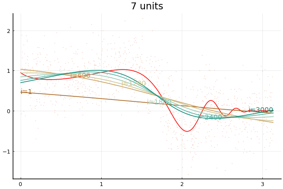
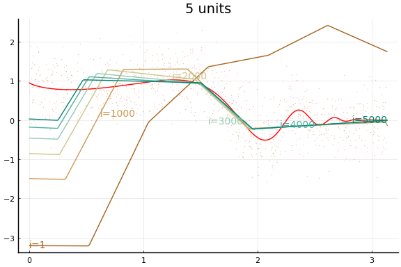
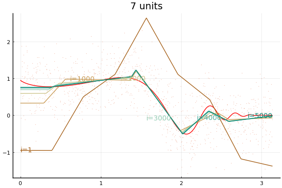
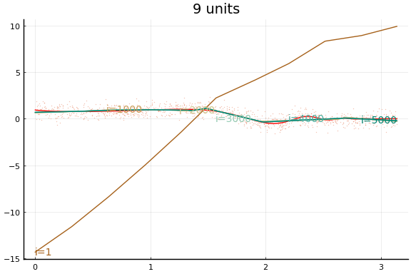
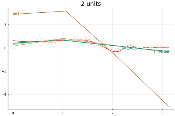
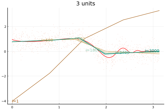
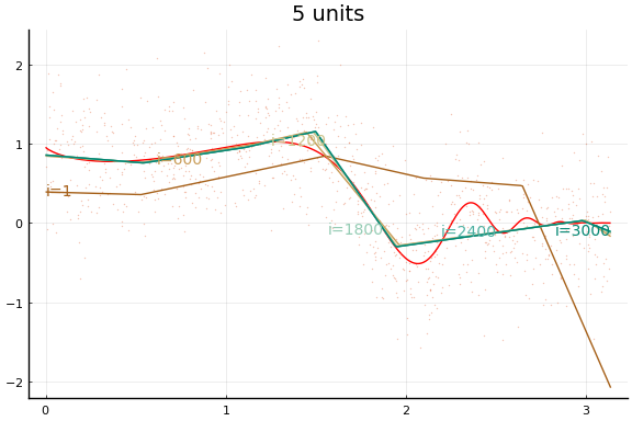
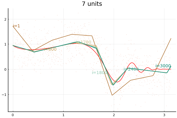
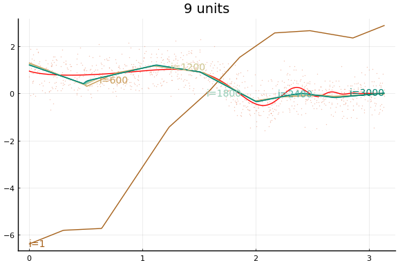
for r in eachindex(rs)
    m,predict,loss = slp(rs[r])
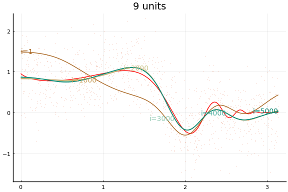
    figs[r]=plot(xg, _f.(xg), lab="True f", title="$(rs[r]) units", color=:red)
    figs[r]=scatter!(x,y, markeralpha=0.4, markersize=1, markerstrokewidth=0, lab="")
    maxiter =500
    opt = Flux.setup(Flux.AMSGrad(),m)
    @time for i = 1:maxiter
        Flux.train!(loss, m, [(x, y)], opt)
        if (i % (maxiter ÷ 5))==0
            l=loss(m, x,y)
            println("$i iteration, loss=$l")
            loc=Int64.(ceil(length(xg)*i/maxiter))
            yg = predict(m,xg)
            figs[r]=plot!(xg,yg, lab="", color=get(cscheme, i/maxiter), alpha=1.0,
                          annotations=(xg[loc], yg[loc],
                                       Plots.text("i=$i", i<maxiter/2 ? :left : :right, pointsize=10,
                                                  color=get(cscheme, i/maxiter)) )
                          )
        end
    end
    display(figs[r])
end

100 iteration, loss=0.39996339084013843
200 iteration, loss=0.36527335501768965
300 iteration, loss=0.35317162062518825
400 iteration, loss=0.34745400528042725
500 iteration, loss=0.34409026968497763
  7.125596 seconds (33.60 M allocations: 1.713 GiB, 2.17% gc time, 99.64% c
ompilation time)
100 iteration, loss=0.39512966167266644
200 iteration, loss=0.3491968668835948
300 iteration, loss=0.3334584539258063
400 iteration, loss=0.3277321878964646
500 iteration, loss=0.3252140534535288
  0.026954 seconds (76.96 k allocations: 174.911 MiB, 48.67% gc time)
100 iteration, loss=0.5459225940487328
200 iteration, loss=0.49455434816234256
300 iteration, loss=0.4591575282748995
400 iteration, loss=0.42610861030831215
500 iteration, loss=0.39688689790684994
  0.024860 seconds (76.96 k allocations: 274.420 MiB, 37.09% gc time)
100 iteration, loss=0.46732713452797275
200 iteration, loss=0.38074800498095346
300 iteration, loss=0.35013412160779467
400 iteration, loss=0.3402542327078661
500 iteration, loss=0.33730003900978134
  0.035528 seconds (76.96 k allocations: 373.923 MiB, 37.77% gc time)
100 iteration, loss=0.3617719038537409
200 iteration, loss=0.34775172920636377
300 iteration, loss=0.34032959420350944
400 iteration, loss=0.33631237116136337
500 iteration, loss=0.3340253656429602
  0.039868 seconds (76.96 k allocations: 473.429 MiB, 34.33% gc time)

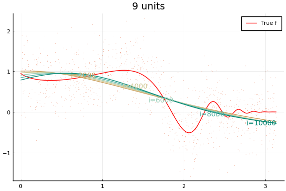
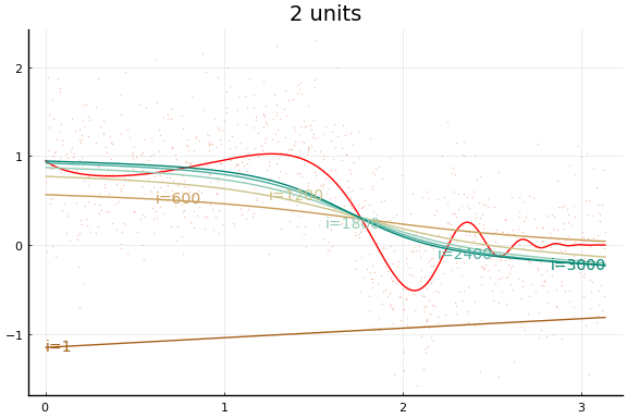
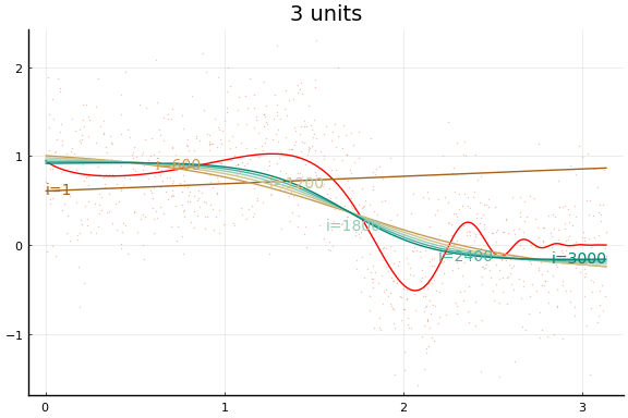
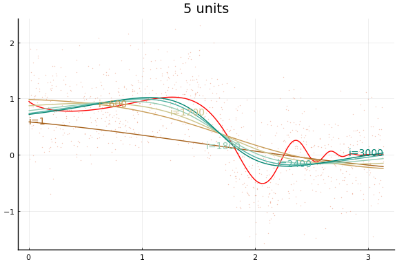
Each invocation of Flux.train! completes one iteration of gradient descent. As you might guess from this API, it is common to train neural networks for a fixed number of iterations instead of until convergence to a local minimum. The number of training iterations can act as a regularization parameter.

Notice how even though a wider network can approximate $f$ better, wider networks also take more training iterations to minimize the loss. This is typical of any minimization algorithm — the number of iterations increases with the problem size.

You may notice that the MSE does not (weakly) decrease with network size. (Or not—both the data and initial values are drawn randomly, and results may vary.) This reflects a problem in the minimization. Care must be used when choosing a minimization algorithm and initial values. We will see more of this below.

Chain interface¶

Flux.jl also contains some higher level functions for creating loss functions for neural networks. Here is the same network as in the previous code block, but using the higher level API.

dimx = 1
figs = Array{typeof(plot(0)),1}(undef,length(rs))
initmfigs = Array{typeof(plot(0)),1}(undef,length(rs))
xt = reshape(Float32.(x), 1, length(x))
yt = reshape(Float32.(y), 1, length(y))
for r in eachindex(rs)
    l = rs[r]
    m = Chain(x->Flux.normalise(x, dims=2),
              Dense(dimx, rs[r], Flux.σ), Dense(rs[r], 1))
    initmfigs[r] = plot(xg, m[1:(end-1)](xg')', lab="", legend=false)
    figs[r]=plot(xg, _f.(xg), lab="", title="$(rs[r]) units", color=:red)
    figs[r]=scatter!(x,y, alpha=0.4, markersize=1, markerstrokewidth=0, lab="")
    maxiter = 500
    opt = Flux.setup(Flux.AMSGrad(),m)
    @time for i = 1:maxiter
        Flux.train!((m,x,y)->Flux.mse(m(x),y), m, [(xt, yt)], opt ) #,
        #cb = Flux.throttle(()->@show(Flux.mse(m(xt),yt)),100))
        if i==1 || (i % (maxiter ÷ 5))==0
            l=Flux.mse(m(xt), yt)
            println("$(rs[r]) units, $i iterations, loss=$l")
            yg = (m(xg'))'
            loc=Int64.(ceil(length(xg)*i/maxiter))
            figs[r]=plot!(xg,yg, lab="", color=get(cscheme, i/maxiter), alpha=1.0,
                          annotations=(xg[loc], yg[loc],
                                       Plots.text("i=$i", i<maxiter/2 ? :left : :right, pointsize=10,
                                                  color=get(cscheme, i/maxiter)) )
                          )
        end
    end
    display(figs[r])
end

2 units, 1 iterations, loss=0.5835158
2 units, 100 iterations, loss=0.37765935
2 units, 200 iterations, loss=0.33820355
2 units, 300 iterations, loss=0.32186928
2 units, 400 iterations, loss=0.31595525
2 units, 500 iterations, loss=0.31357348
  8.587543 seconds (34.99 M allocations: 1.678 GiB, 1.73% gc time, 99.52% c
ompilation time)
3 units, 1 iterations, loss=0.41534433
3 units, 100 iterations, loss=0.33576682
3 units, 200 iterations, loss=0.33468783
3 units, 300 iterations, loss=0.33384335
3 units, 400 iterations, loss=0.33315718
3 units, 500 iterations, loss=0.3326006
  0.045901 seconds (256.02 k allocations: 63.018 MiB, 26.26% gc time)
5 units, 1 iterations, loss=0.56019837
5 units, 100 iterations, loss=0.35969394
5 units, 200 iterations, loss=0.33136117
5 units, 300 iterations, loss=0.32759973
5 units, 400 iterations, loss=0.32617292
5 units, 500 iterations, loss=0.32490262
  0.049912 seconds (256.02 k allocations: 74.522 MiB, 22.81% gc time)
7 units, 1 iterations, loss=2.610366
7 units, 100 iterations, loss=0.3360725
7 units, 200 iterations, loss=0.33046693
7 units, 300 iterations, loss=0.32976365
7 units, 400 iterations, loss=0.32894534
7 units, 500 iterations, loss=0.3279586
  0.057034 seconds (256.02 k allocations: 86.050 MiB, 24.45% gc time)
9 units, 1 iterations, loss=2.3100607
9 units, 100 iterations, loss=0.35537902
9 units, 200 iterations, loss=0.33313772
9 units, 300 iterations, loss=0.33063537
9 units, 400 iterations, loss=0.32995462
9 units, 500 iterations, loss=0.32940575
  0.061050 seconds (256.02 k allocations: 97.554 MiB, 25.91% gc time)

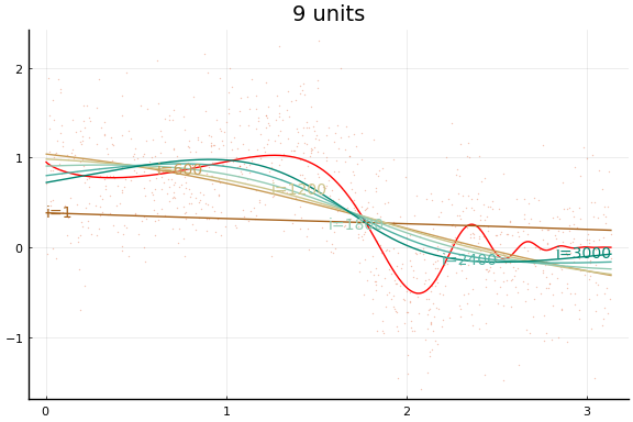
The figures do not appear identical to the first example since the initial values differ, and the above code first normalises the $x$s.

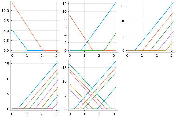
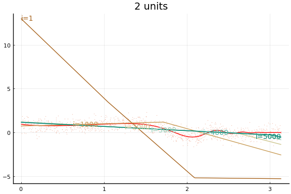
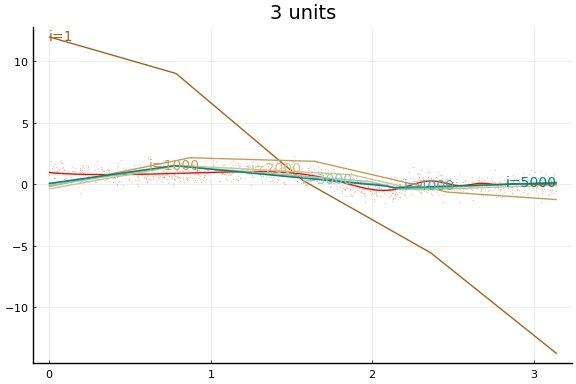
Initial values¶

Initial values are especially important with neural networks because activation functions tend to be flat at the extremes. This causes the gradient of the loss function to vanish in some regions of the parameter space. For gradient descent to be successful, it is important to avoid regions with vanishing gradients. The default initial values of $w$ and $b$ used by Flux tend to work better with normalised $x$. The initial activation are shown below.

plot(initmfigs..., legend=false)

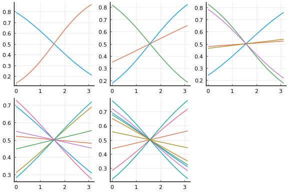
At these initial values, $w’x + b$, does change sign for each activation, but $w’x$ is small enough that $\psi(w’x + b)$ is approximately linear. This will make it initially difficult to distinguish $\beta \psi’$ from $w$,

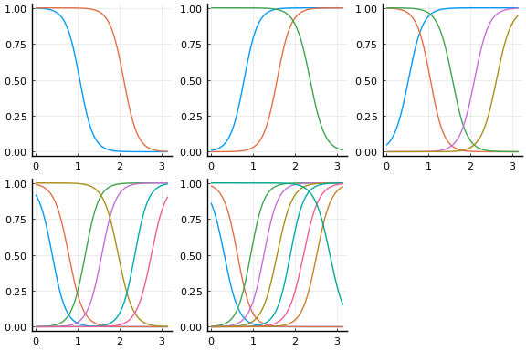
We can improve the fit by choosing initial values more carefully. The following code choses initial $w$ and $b$ to make sure the activation functions vary nonlinearly in the support of $x$. The initial activations functions are plotted below.

dimx = 1
figs = Array{typeof(plot(0)),1}(undef,length(rs))
initmfigs = Array{typeof(plot(0)),1}(undef,length(rs))
xt = reshape(Float32.(x), 1, length(x))
yt = reshape(Float32.(y), 1, length(y))
for r in eachindex(rs)
  l = rs[r]
  m = Chain(Dense(dimx, l, Flux.σ), Dense(rs[r], 1))
  # adjust initial weights to make sure each node is nonlinear in support of X
  m[1].weight .= -m[1].weight .+ sign.(m[1].weight)*2*π
  # adjust initial intercepts to be in the support of w*x
  m[1].bias .= -m[1].bias .- m[1].weight[:].*(π/(l+1):π/(l+1):π*l/(l+1))
  # make initial output weights optimal given first layer
  X = vcat(1, m[1](xt))
  bols = (X*X') \ (X*y)
  m[2].weight .= -m[2].weight .+ bols[2:end]'
  m[2].bias .= -m[2].bias .- mean(m(xt) .- yt)
  initmfigs[r] = plot(xg, m[1](xg')', lab="", legend=false)
  figs[r]=plot(xg, _f.(xg), lab="", title="$(rs[r]) units", color=:red)
  figs[r]=scatter!(x,y, alpha=0.4, markersize=1, markerstrokewidth=0, lab="")
  maxiter = 500
  opt = Flux.setup(Flux.AMSGrad(),m)
  @time for i = 1:maxiter
    Flux.train!((m,x,y)->Flux.mse(m(x),y), m, [(xt, yt)], opt ) #,
    #cb = Flux.throttle(()->@show(Flux.mse(m(xt),yt)),100))
    if i==1 || (i % (maxiter ÷ 5))==0
      l=Flux.mse(m(xt), yt)
      println("$(rs[r]) units, $i iterations, loss=$l")
      yg = m(xg')'
      loc=Int64.(ceil(length(xg)*i/maxiter))
      figs[r]=plot!(xg,yg, lab="", color=get(cscheme, i/maxiter), alpha=1.0,
                    annotations=(xg[loc], yg[loc],
                                 Plots.text("i=$i", i<maxiter/2 ? :left : :right, pointsize=10,
                                            color=get(cscheme, i/maxiter)) )
                    )
    end
  end
end
nothing

2 units, 1 iterations, loss=0.47121212
2 units, 100 iterations, loss=0.3478092
2 units, 200 iterations, loss=0.31684136
2 units, 300 iterations, loss=0.301511
2 units, 400 iterations, loss=0.29349726
2 units, 500 iterations, loss=0.28903913
  0.484956 seconds (3.00 M allocations: 170.878 MiB, 4.35% gc time, 93.50% 
compilation time)
3 units, 1 iterations, loss=0.83332896
3 units, 100 iterations, loss=0.38979414
3 units, 200 iterations, loss=0.3194255
3 units, 300 iterations, loss=0.29777384
3 units, 400 iterations, loss=0.28810304
3 units, 500 iterations, loss=0.28242868
  0.026664 seconds (139.36 k allocations: 40.936 MiB, 24.01% gc time)
5 units, 1 iterations, loss=0.31125516
5 units, 100 iterations, loss=0.25697738
5 units, 200 iterations, loss=0.25488177
5 units, 300 iterations, loss=0.25366494
5 units, 400 iterations, loss=0.2528164
5 units, 500 iterations, loss=0.25218457
  0.028785 seconds (139.36 k allocations: 52.440 MiB, 13.68% gc time)
7 units, 1 iterations, loss=0.27260572
7 units, 100 iterations, loss=0.25034013
7 units, 200 iterations, loss=0.24807897
7 units, 300 iterations, loss=0.2472352
7 units, 400 iterations, loss=0.24678983
7 units, 500 iterations, loss=0.24648862
  0.038980 seconds (139.36 k allocations: 63.967 MiB, 26.02% gc time)
9 units, 1 iterations, loss=0.35958824
9 units, 100 iterations, loss=0.24537204
9 units, 200 iterations, loss=0.24433525
9 units, 300 iterations, loss=0.24386269
9 units, 400 iterations, loss=0.2435471
9 units, 500 iterations, loss=0.24333371
  0.043938 seconds (139.36 k allocations: 75.471 MiB, 26.40% gc time)

display(plot(initmfigs..., legend=false))

And the fit figures.

for f in figs
  display(f)
end

We can see that the training is now much more successful. Choosing initial values carefully was very helpful.

Rectified linear¶

Large applications of neural networks often use rectified linear activation for efficiency. Let’s see how the same example behaves with (leaky) rectified linear activation.

dimx = 1
figs = Array{typeof(plot(0)),1}(undef,length(rs))
for r in eachindex(rs)
  l = rs[r]
  m = Chain(Dense(dimx, rs[r], Flux.leakyrelu), Dense(rs[r], 1)) # notice the change
  # adjust initial weights to make sure each node is nonlinear in support of X
  m[1].weight .= -m[1].weight .+ sign.(m[1].weight)*2*π
  # adjust initial intercepts to be in the support of w*x
  m[1].bias .= -m[1].bias .- m[1].weight[:].*(π/(l+1):π/(l+1):π*l/(l+1))
  # make initial output weights optimal given first layer
  X = vcat(1, m[1](xt))
  bols = (X*X') \ (X*y)
  m[2].weight .= -m[2].weight .+ bols[2:end]'
  m[2].bias .= -m[2].bias .- mean(m(xt) .- yt)
  initmfigs[r] = plot(xg, m[1:(end-1)](xg')', lab="", legend=false)
  figs[r]=plot(xg, _f.(xg), lab="", title="$(rs[r]) units", color=:red)
  figs[r]=scatter!(x,y, alpha=0.4, markersize=1, markerstrokewidth=0, lab="")
  maxiter = 1000
  opt=Flux.setup(Flux.AMSGrad(),m)
  @time for i = 1:maxiter
    Flux.train!((m,x,y)->Flux.mse(m(x),y), m, [(xt, yt)], opt ) #,
                #cb = Flux.throttle(()->@show(Flux.mse(m(xt),yt)),100))
    if i==1 || (i % (maxiter ÷ 5))==0
      l=Flux.mse(m(xt), yt)
      println("$(rs[r]) units, $i iterations, loss=$l")
      yg = m(xg')'
      loc=Int64.(ceil(length(xg)*i/maxiter))
      figs[r]=plot!(xg,yg, lab="", color=get(cscheme, i/maxiter), alpha=1.0,
                    annotations=(xg[loc], yg[loc],
                                 Plots.text("i=$i", i<maxiter/2 ? :left : :right, pointsize=10,
                                            color=get(cscheme, i/maxiter)) )
                    )
    end
  end
end
display(plot(initmfigs..., legend=false) )

for f in figs
  display(f)
end

2 units, 1 iterations, loss=22.61312
2 units, 200 iterations, loss=6.576372
2 units, 400 iterations, loss=4.649459
2 units, 600 iterations, loss=3.5492566
2 units, 800 iterations, loss=2.804766
2 units, 1000 iterations, loss=2.260517
  0.805275 seconds (4.28 M allocations: 257.244 MiB, 3.22% gc time, 94.00% 
compilation time)
3 units, 1 iterations, loss=1.7244341
3 units, 200 iterations, loss=0.43364766
3 units, 400 iterations, loss=0.36388764
3 units, 600 iterations, loss=0.33708185
3 units, 800 iterations, loss=0.32145885
3 units, 1000 iterations, loss=0.31237894
  0.040428 seconds (284.85 k allocations: 81.818 MiB, 20.96% gc time)
5 units, 1 iterations, loss=2.0703168
5 units, 200 iterations, loss=0.27558643
5 units, 400 iterations, loss=0.26430288
5 units, 600 iterations, loss=0.25806376
5 units, 800 iterations, loss=0.25452963
5 units, 1000 iterations, loss=0.25266287
  0.049822 seconds (284.85 k allocations: 104.766 MiB, 31.45% gc time)
7 units, 1 iterations, loss=12.762251
7 units, 200 iterations, loss=0.27903998
7 units, 400 iterations, loss=0.26031134
7 units, 600 iterations, loss=0.25402334
7 units, 800 iterations, loss=0.2506849
7 units, 1000 iterations, loss=0.24845254
  0.054245 seconds (284.85 k allocations: 127.760 MiB, 33.05% gc time)
9 units, 1 iterations, loss=2.3123422
9 units, 200 iterations, loss=0.2597074
9 units, 400 iterations, loss=0.25246483
9 units, 600 iterations, loss=0.24929576
9 units, 800 iterations, loss=0.24769343
9 units, 1000 iterations, loss=0.2468164
  0.056090 seconds (284.85 k allocations: 150.708 MiB, 37.05% gc time)

Stochastic Gradient descent¶

The above examples all used the full data in each iteration of gradient descent. Computation can be reduced and the parameter space can possibly be explored more by using stochastic gradient descent. In stochastic gradient descent, a subset (possibly even of size 1) of the data is used to compute the gradient for each iteration. To accomplish this in Flux, we should give the Flux.train! function an array of tuples of data consisting of the subsets to be used in iteration. Each call to Flux.train! loops over all tuples of data, doing one gradient descent iteration for each. This whole process is referred to as a training epoch. You could use (the below does not) Flux’s @epochs macro for running multiple training epochs without writing a loop.

dimx = 1
figs = Array{typeof(plot(0)),1}(undef,length(rs))
for r in eachindex(rs)
  l = rs[r]
  m = Chain(Dense(dimx, rs[r], Flux.leakyrelu), Dense(rs[r], 1)) # notice the change
  # adjust initial weights to make sure each node is nonlinear in support of X
  m[1].weight .= -m[1].weight .+ sign.(m[1].weight)*2*π
  # adjust initial intercepts to be in the support of w*x
  m[1].bias .= -m[1].bias .- m[1].weight[:].*(π/(l+1):π/(l+1):π*l/(l+1))
  # make initial output weights optimal given first layer
  X = vcat(1, m[1](xt))
  bols = (X*X') \ (X*y)
  m[2].weight .= -m[2].weight .+ bols[2:end]'
  m[2].bias .= -m[2].bias .- mean(m(xt) .- yt)
  initmfigs[r] = plot(xg, m[1:(end-1)](xg')', lab="", legend=false)
  figs[r]=plot(xg, _f.(xg), lab="", title="$(rs[r]) units", color=:red)
  figs[r]=scatter!(x,y, alpha=0.4, markersize=1, markerstrokewidth=0, lab="")
  maxiter = 1000
  opt = Flux.setup(Flux.AMSGrad(),m)
  @time for i = 1:maxiter
    Flux.train!((m,x,y)->Flux.mse(m(x),y), m,
                # partition data into 100 batches
                [(xt[:,p], yt[:,p]) for p in Base.Iterators.partition(1:length(y), 100)],
                opt ) #,
    if i==1 || (i % (maxiter ÷ 5))==0
      l=Flux.mse(m(xt), yt)
      println("$(rs[r]) units, $i iterations, loss=$l")
      yg = m(xg')'
      loc=Int64.(ceil(length(xg)*i/maxiter))
      figs[r]=plot!(xg,yg, lab="", color=get(cscheme, i/maxiter), alpha=1.0,
                    annotations=(xg[loc], yg[loc],
                                 Plots.text("i=$i", i<maxiter/2 ? :left : :right, pointsize=10,
                                            color=get(cscheme, i/maxiter)) )
                    )
    end
  end
end

for f in figs
  display(f)
end

2 units, 1 iterations, loss=11.173492
2 units, 200 iterations, loss=0.3890759
2 units, 400 iterations, loss=0.33853266
2 units, 600 iterations, loss=0.33775446
2 units, 800 iterations, loss=0.33768705
2 units, 1000 iterations, loss=0.3376491
  0.445585 seconds (3.61 M allocations: 337.168 MiB, 6.73% gc time, 58.73% 
compilation time)
3 units, 1 iterations, loss=2.013808
3 units, 200 iterations, loss=0.3171627
3 units, 400 iterations, loss=0.30799368
3 units, 600 iterations, loss=0.2779722
3 units, 800 iterations, loss=0.26881906
3 units, 1000 iterations, loss=0.2635552
  0.193676 seconds (2.76 M allocations: 307.136 MiB, 17.06% gc time)
5 units, 1 iterations, loss=0.6147741
5 units, 200 iterations, loss=0.24580134
5 units, 400 iterations, loss=0.24449614
5 units, 600 iterations, loss=0.24442013
5 units, 800 iterations, loss=0.24435247
5 units, 1000 iterations, loss=0.24432306
  0.208325 seconds (2.76 M allocations: 329.627 MiB, 17.77% gc time)
7 units, 1 iterations, loss=7.8050523
7 units, 200 iterations, loss=0.262305
7 units, 400 iterations, loss=0.25340876
7 units, 600 iterations, loss=0.2495587
7 units, 800 iterations, loss=0.24680258
7 units, 1000 iterations, loss=0.24566627
  0.231164 seconds (2.79 M allocations: 353.720 MiB, 18.70% gc time)
9 units, 1 iterations, loss=6.610447
9 units, 200 iterations, loss=0.28529337
9 units, 400 iterations, loss=0.25992322
9 units, 600 iterations, loss=0.25541195
9 units, 800 iterations, loss=0.25325322
9 units, 1000 iterations, loss=0.2522086
  0.223981 seconds (2.79 M allocations: 377.584 MiB, 20.85% gc time)

Here we see an in sample MSE about as low as the best previous result. Note, however, the longer training time. Each “iteration” above is an epoch, which consists of 10 gradient descent steps using the 10 different subsets (or batches) of data of size 100.

Rate of convergence¶

• (Chen and White 1999)⁴
• $f(x) = \Er[y|x]$ with Fourier representation $$f(x) = \int e^{i a'x} d\sigma_f(a)$$ where $\int (\sqrt{a’a} \vee 1) d|\sigma_f|(a) < \infty$
• Network sieve : $$\begin{align*} \mathcal{G}_n = \{ & g: g(x) = \sum_{j=1}^{r_n} \beta_j (a_j'a_j \vee 1)^{-1} \psi(a_j'x + b_j), \\ & \norm{\beta}_1 \leq B_n \} \end{align*}$$

The setup in (Chen and White 1999)⁴ is more general. They consider estimating both $f$ and its first $m$ derivatives. Here, we focus on the case of just estimating $f$. (Chen and White 1999)⁴ also consider estimation of functions other than conditional expectations.

The restriction on $f$ in the second bullet is used to control approximation error. The second bullet says that $f$ is the inverse Fourier transform of measure $\sigma_f$. The bite of the restriction on $f$ comes from the requirement that $\sigma_f$ be absolutely integral, $\int (\sqrt{a’a} \vee 1) d|\sigma_f|(a) < \infty$. It would be a good exercise to check whether this restriction is satisfied by some familiar types of functions. (Barron 1993)⁵ first showed that neural networks approximate this class of functions well, and compares the approximation rate of neural networks to other function approximation results.

• See (Farrell, Liang, and Misra 2021)⁶ for more contemporary approach, applicable to currently used network architectures

References¶