
This work is licensed under a Creative Commons Attribution-ShareAlike 4.0 International License
using CovidSEIR,  Plots, DataFrames, JLD2, StatsPlots, MCMCChains
Plots.pyplot()
jmddir = normpath(joinpath(dirname(Base.find_package("CovidSEIR")),"..","docs","jmd"))
covdf = covidjhudata();
Canada
We estimate the model with the following code. It takes about an hour.
canada = CountryData(covdf, "Canada");
using Turing
canmod = CovidSEIR.TimeVarying.countrymodel(canada)
cc = Turing.psample(canmod, NUTS(0.65), 5000, 4)
import JLD2
JLD2.@save "$jmddir/canada_$(Dates.today()).jld2" cc
JLD2.@load "$jmddir/canada_dhmc_2020-04-13.jld2" cc dayt0;
cc = MCMCChains.Chains(collect(cc.value.data), replace.(cc.name_map.parameters, r"([^\[])([1-9])" => s"\1[\2]"))
Object of type Chains, with data of type 5000×15×4 Array{Float64,3}

Iterations        = 1:5000
Thinning interval = 1
Chains            = 1, 2, 3, 4
Samples per chain = 5000
parameters        = τ, sigD, sigC, sigRc, a, pE0, p[1], p[2], β[1], β[2], β
[3], γ[1], γ[2], ρ[1], ρ[2]

2-element Array{MCMCChains.ChainDataFrame,1}

Summary Statistics
  parameters      mean       std  naive_se    mcse       ess   r_hat
  ──────────  ────────  ────────  ────────  ──────  ────────  ──────
           τ    0.2357    0.6185    0.0044  0.0434   80.3213  2.7437
        sigD    6.5869    0.8252    0.0058  0.0488   84.3120  1.2775
        sigC  663.0470  132.2966    0.9355  8.8404   80.3213  2.0702
       sigRc  109.1233    8.8844    0.0628  0.4840  122.8527  1.1655
           a    0.6428    0.2756    0.0019  0.0193   80.3213  2.8064
         pE0    0.0000    0.0000    0.0000  0.0000   80.3213  1.8518
        p[1]    0.0819    0.2048    0.0014  0.0143   80.3213  2.3034
        p[2]    0.0054    0.0035    0.0000  0.0002   80.3213  4.0799
        β[1]    0.2341    0.2845    0.0020  0.0186   80.3213  1.3055
        β[2]    0.6854    0.5439    0.0038  0.0373   80.3213  1.8702
        β[3]    3.4579    0.8677    0.0061  0.0608   80.3213  2.7532
        γ[1]    2.1268    1.0667    0.0075  0.0754   80.3213  4.6674
        γ[2]    0.0439    0.0157    0.0001  0.0011   80.3213  3.1084
        ρ[1]    0.2345    0.3476    0.0025  0.0244   80.3213  4.3679
        ρ[2]   56.7301   23.8913    0.1689  1.6324   80.3213  1.8519

Quantiles
  parameters      2.5%     25.0%     50.0%     75.0%     97.5%
  ──────────  ────────  ────────  ────────  ────────  ────────
           τ    0.0000    0.0000    0.0001    0.0010    2.2230
        sigD    5.2897    6.0577    6.3179    7.1150    8.5042
        sigC  340.9755  643.1188  676.1973  738.0302  872.2481
       sigRc   92.9782  103.0199  110.7701  112.5595  129.1059
           a    0.1631    0.3985    0.6762    0.9309    0.9894
         pE0    0.0000    0.0000    0.0000    0.0000    0.0000
        p[1]    0.0028    0.0038    0.0044    0.0163    0.8283
        p[2]    0.0039    0.0040    0.0041    0.0041    0.0163
        β[1]    0.0000    0.0002    0.0995    0.4113    0.8889
        β[2]    0.0241    0.1801    0.5443    1.3260    1.5558
        β[3]    1.2217    3.3502    3.6691    3.9622    4.6629
        γ[1]    0.0171    2.2217    2.6733    2.7457    2.9976
        γ[2]    0.0338    0.0380    0.0381    0.0401    0.0932
        ρ[1]    0.0000    0.0004    0.0050    0.5601    0.9289
        ρ[2]   24.6373   24.7181   67.2189   71.7995   99.9910
Estimates
plot(cc)
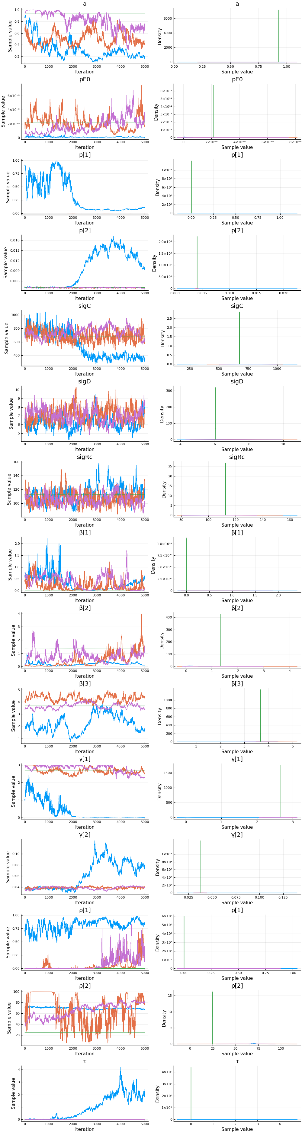
We can see that there might be convergence issues. There are large differences between the four chains for some parameters.
describe(cc)
2-element Array{MCMCChains.ChainDataFrame,1}

Summary Statistics
  parameters      mean       std  naive_se    mcse       ess   r_hat
  ──────────  ────────  ────────  ────────  ──────  ────────  ──────
           τ    0.2357    0.6185    0.0044  0.0434   80.3213  2.7437
        sigD    6.5869    0.8252    0.0058  0.0488   84.3120  1.2775
        sigC  663.0470  132.2966    0.9355  8.8404   80.3213  2.0702
       sigRc  109.1233    8.8844    0.0628  0.4840  122.8527  1.1655
           a    0.6428    0.2756    0.0019  0.0193   80.3213  2.8064
         pE0    0.0000    0.0000    0.0000  0.0000   80.3213  1.8518
        p[1]    0.0819    0.2048    0.0014  0.0143   80.3213  2.3034
        p[2]    0.0054    0.0035    0.0000  0.0002   80.3213  4.0799
        β[1]    0.2341    0.2845    0.0020  0.0186   80.3213  1.3055
        β[2]    0.6854    0.5439    0.0038  0.0373   80.3213  1.8702
        β[3]    3.4579    0.8677    0.0061  0.0608   80.3213  2.7532
        γ[1]    2.1268    1.0667    0.0075  0.0754   80.3213  4.6674
        γ[2]    0.0439    0.0157    0.0001  0.0011   80.3213  3.1084
        ρ[1]    0.2345    0.3476    0.0025  0.0244   80.3213  4.3679
        ρ[2]   56.7301   23.8913    0.1689  1.6324   80.3213  1.8519

Quantiles
  parameters      2.5%     25.0%     50.0%     75.0%     97.5%
  ──────────  ────────  ────────  ────────  ────────  ────────
           τ    0.0000    0.0000    0.0001    0.0010    2.2230
        sigD    5.2897    6.0577    6.3179    7.1150    8.5042
        sigC  340.9755  643.1188  676.1973  738.0302  872.2481
       sigRc   92.9782  103.0199  110.7701  112.5595  129.1059
           a    0.1631    0.3985    0.6762    0.9309    0.9894
         pE0    0.0000    0.0000    0.0000    0.0000    0.0000
        p[1]    0.0028    0.0038    0.0044    0.0163    0.8283
        p[2]    0.0039    0.0040    0.0041    0.0041    0.0163
        β[1]    0.0000    0.0002    0.0995    0.4113    0.8889
        β[2]    0.0241    0.1801    0.5443    1.3260    1.5558
        β[3]    1.2217    3.3502    3.6691    3.9622    4.6629
        γ[1]    0.0171    2.2217    2.6733    2.7457    2.9976
        γ[2]    0.0338    0.0380    0.0381    0.0401    0.0932
        ρ[1]    0.0000    0.0004    0.0050    0.5601    0.9289
        ρ[2]   24.6373   24.7181   67.2189   71.7995   99.9910
The parameter estimates are generally not very precise.
Fit
sdf = simtrajectories(cc, canada, 1:200)
f = plotvars(sdf, canada)
f.fit
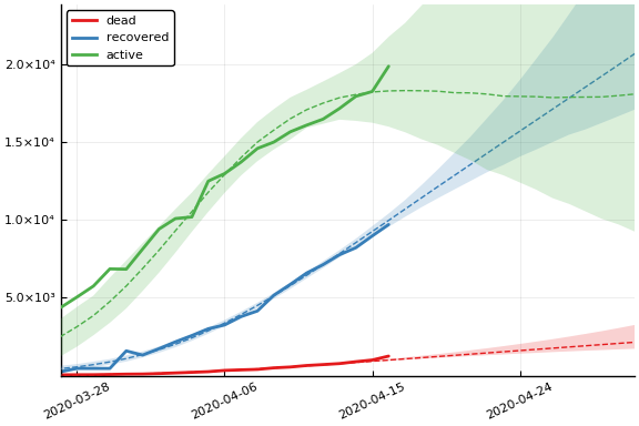
In this figure, solid lines are observed data, dashed lines are posterior means, and the shaded region is a pointwise 90% credible interval.
Implications
We now look at the model’s projections for some observed and unobserved variables.
for fig in f.trajectories
  display(fig)
end
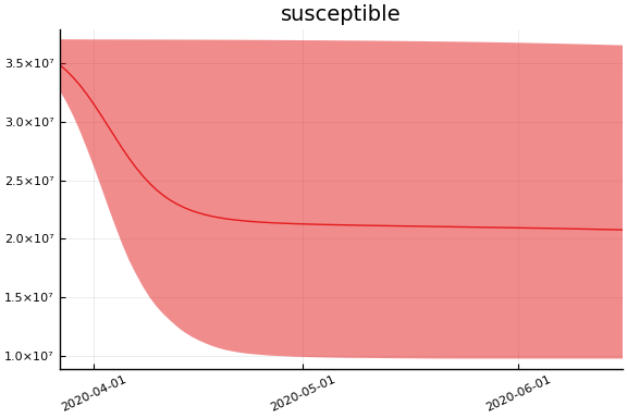
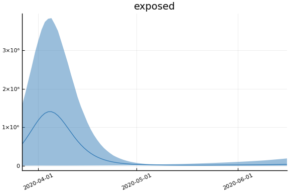
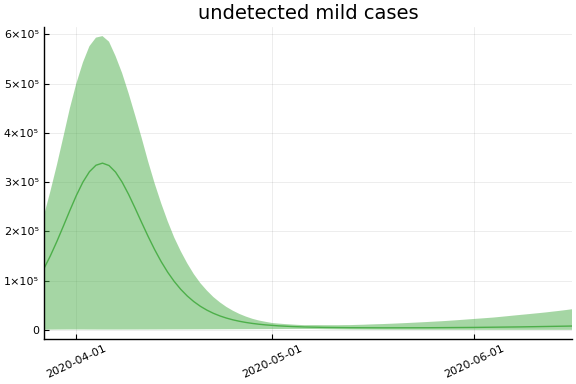
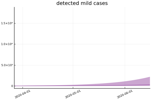
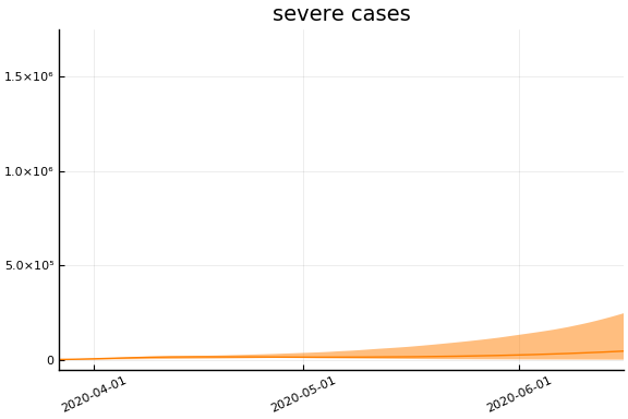
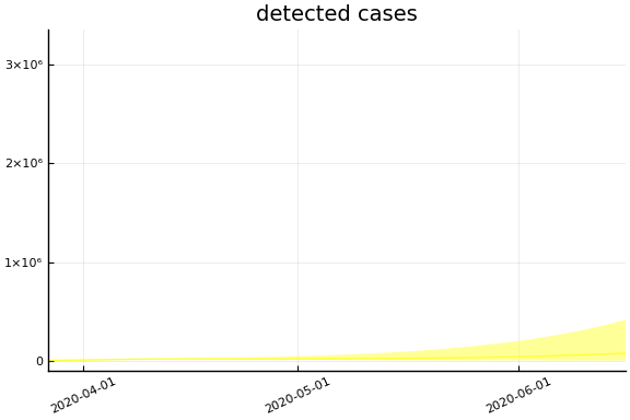
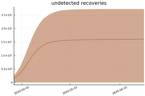
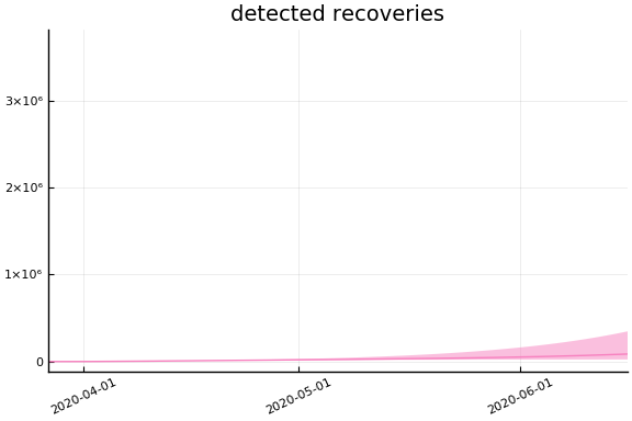
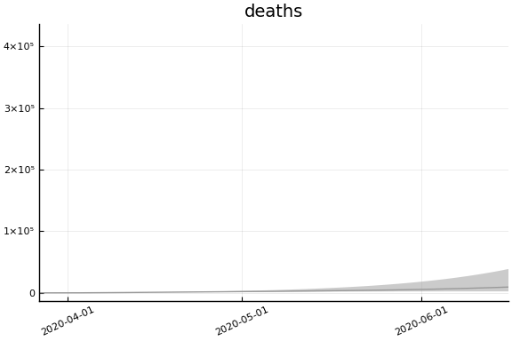
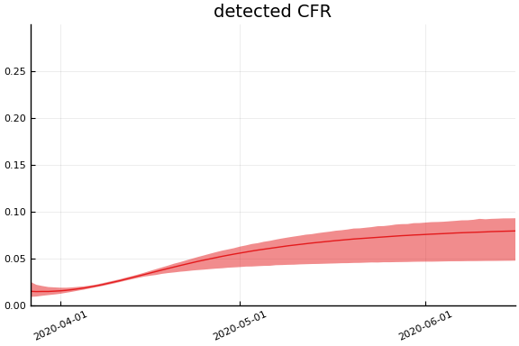
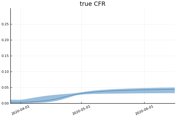
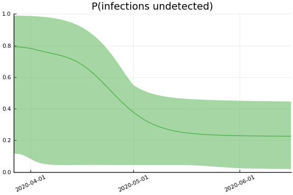
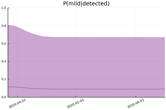
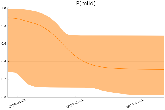
In general we see a similar pattern as noted above: the posteriors for observed variables are fairly precise. However, the posteriors for unobserved variables, such as the portion of undetected infections and the portion of mild infections, are very imprecise.