This work is licensed under a Creative Commons Attribution-ShareAlike 4.0 International License
using CovidSEIR,  Plots, DataFrames, JLD2, StatsPlots, MCMCChains
Plots.pyplot()
jmddir = normpath(joinpath(dirname(Base.find_package("CovidSEIR")),"..","docs","jmd"))
covdf = covidjhudata();
South Korea
korea = CountryData(covdf, "Korea, South")
CovidSEIR.CountryData{Float64,Int64}(5.1635256e7, [1, 2, 3, 4, 5, 6, 7, 8,
9, 10  …  77, 78, 79, 80, 81, 82, 83, 84, 85, 86], [0.0, 0.0, 0.0, 0.0, 0.0
, 0.0, 0.0, 0.0, 0.0, 0.0  …  192.0, 200.0, 204.0, 208.0, 211.0, 214.0, 217
.0, 222.0, 225.0, 229.0], [0.0, 0.0, 0.0, 0.0, 0.0, 0.0, 0.0, 0.0, 0.0, 0.0
  …  6694.0, 6776.0, 6973.0, 7117.0, 7243.0, 7368.0, 7447.0, 7534.0, 7616.0
, 7757.0], [1.0, 1.0, 2.0, 2.0, 3.0, 4.0, 4.0, 4.0, 4.0, 11.0  …  3445.0, 3
408.0, 3246.0, 3125.0, 3026.0, 2930.0, 2873.0, 2808.0, 2750.0, 2627.0])
using Turing
mdl = CovidSEIR.TimeVarying.countrymodel(korea)
cc = Turing.psample(mdl, NUTS(0.65), 5000, 4)
import JLD2
JLD2.@save "$jmddir/korea_tv_$(Dates.today()).jld2" cc
JLD2.@load "$jmddir/korea_dhmc_2020-04-13.jld2" cc dayt0;
cc = MCMCChains.Chains(collect(cc.value.data), replace.(cc.name_map.parameters, r"([^\[])([1-9])" => s"\1[\2]"))
Object of type Chains, with data of type 5000×15×4 Array{Float64,3}

Iterations        = 1:5000
Thinning interval = 1
Chains            = 1, 2, 3, 4
Samples per chain = 5000
parameters        = τ, sigD, sigC, sigRc, a, pE0, p[1], p[2], β[1], β[2], β
[3], γ[1], γ[2], ρ[1], ρ[2]

2-element Array{MCMCChains.ChainDataFrame,1}

Summary Statistics
  parameters      mean       std  naive_se     mcse      ess   r_hat
  ──────────  ────────  ────────  ────────  ───────  ───────  ──────
           τ    0.0146    0.0597    0.0004   0.0041  80.3213  1.3408
        sigD    5.3642    2.4216    0.0171   0.1694  80.3213  5.0384
        sigC  951.3287  978.9917    6.9225  69.0719  80.3213  2.2197
       sigRc  845.4857  105.0627    0.7429   5.9862  80.3213  1.4793
           a    0.5215    0.2690    0.0019   0.0176  80.3213  1.8935
         pE0    0.0002    0.0005    0.0000   0.0000  80.3213  1.4380
        p[1]    0.0316    0.0626    0.0004   0.0044  80.3213  2.4790
        p[2]    0.0031    0.0089    0.0001   0.0006  80.3213  1.2621
        β[1]    0.7778    0.8358    0.0059   0.0555  80.3213  1.4458
        β[2]    0.6354    0.7074    0.0050   0.0398  80.3370  1.2070
        β[3]    2.0175    1.3794    0.0098   0.0966  80.3213  3.3188
        γ[1]    1.5137    1.1407    0.0081   0.0801  80.3213  3.0029
        γ[2]    0.0515    0.0970    0.0007   0.0068  80.3213  1.3837
        ρ[1]    0.5549    0.2274    0.0016   0.0136  80.3213  1.3732
        ρ[2]   47.0605   11.1717    0.0790   0.7350  80.3213  1.2892

Quantiles
  parameters      2.5%     25.0%     50.0%      75.0%      97.5%
  ──────────  ────────  ────────  ────────  ─────────  ─────────
           τ    0.0000    0.0000    0.0000     0.0001     0.2457
        sigD    2.4786    2.9594    5.5550     7.6868     8.8722
        sigC  217.4268  265.3300  550.1108  1232.7812  4068.7156
       sigRc  673.8938  765.5432  836.1810   916.0544  1064.8168
           a    0.0746    0.3490    0.5506     0.7427     0.9411
         pE0    0.0000    0.0000    0.0000     0.0000     0.0016
        p[1]    0.0000    0.0001    0.0003     0.0240     0.2330
        p[2]    0.0008    0.0008    0.0008     0.0009     0.0354
        β[1]    0.0000    0.0026    0.5025     1.2954     2.8868
        β[2]    0.0000    0.0583    0.3820     1.0063     2.4575
        β[3]    0.0405    0.7791    1.7061     3.3934     4.2446
        γ[1]    0.0316    0.5668    1.1303     3.0000     3.0000
        γ[2]    0.0214    0.0264    0.0275     0.0286     0.4204
        ρ[1]    0.1889    0.3367    0.5769     0.7514     0.9503
        ρ[2]   28.7635   38.8180   46.5332    53.4753    75.3812
Estimates
plot(cc)
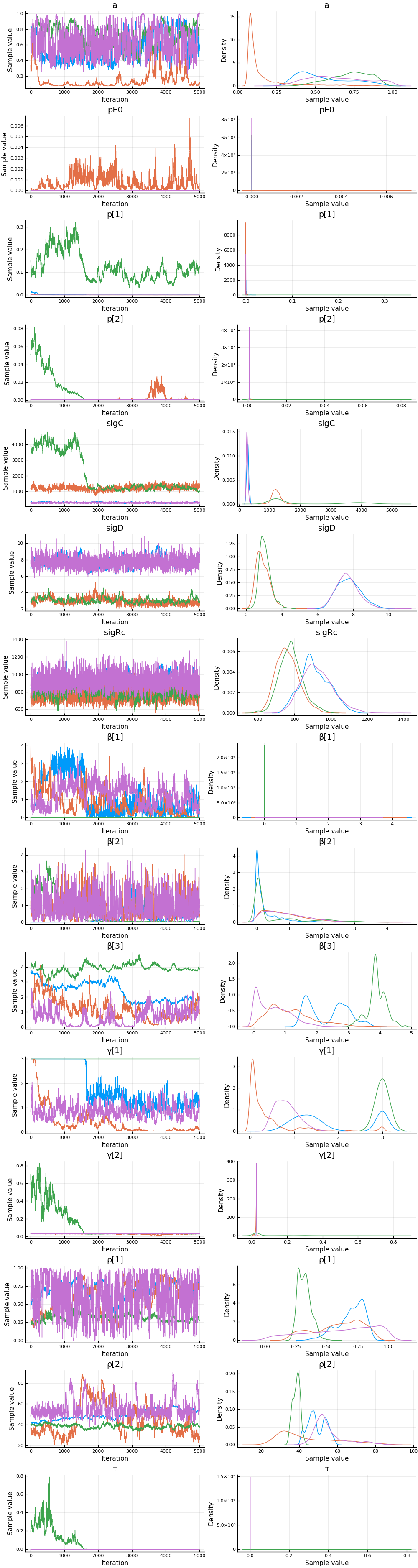
describe(cc)
2-element Array{MCMCChains.ChainDataFrame,1}

Summary Statistics
  parameters      mean       std  naive_se     mcse      ess   r_hat
  ──────────  ────────  ────────  ────────  ───────  ───────  ──────
           τ    0.0146    0.0597    0.0004   0.0041  80.3213  1.3408
        sigD    5.3642    2.4216    0.0171   0.1694  80.3213  5.0384
        sigC  951.3287  978.9917    6.9225  69.0719  80.3213  2.2197
       sigRc  845.4857  105.0627    0.7429   5.9862  80.3213  1.4793
           a    0.5215    0.2690    0.0019   0.0176  80.3213  1.8935
         pE0    0.0002    0.0005    0.0000   0.0000  80.3213  1.4380
        p[1]    0.0316    0.0626    0.0004   0.0044  80.3213  2.4790
        p[2]    0.0031    0.0089    0.0001   0.0006  80.3213  1.2621
        β[1]    0.7778    0.8358    0.0059   0.0555  80.3213  1.4458
        β[2]    0.6354    0.7074    0.0050   0.0398  80.3370  1.2070
        β[3]    2.0175    1.3794    0.0098   0.0966  80.3213  3.3188
        γ[1]    1.5137    1.1407    0.0081   0.0801  80.3213  3.0029
        γ[2]    0.0515    0.0970    0.0007   0.0068  80.3213  1.3837
        ρ[1]    0.5549    0.2274    0.0016   0.0136  80.3213  1.3732
        ρ[2]   47.0605   11.1717    0.0790   0.7350  80.3213  1.2892

Quantiles
  parameters      2.5%     25.0%     50.0%      75.0%      97.5%
  ──────────  ────────  ────────  ────────  ─────────  ─────────
           τ    0.0000    0.0000    0.0000     0.0001     0.2457
        sigD    2.4786    2.9594    5.5550     7.6868     8.8722
        sigC  217.4268  265.3300  550.1108  1232.7812  4068.7156
       sigRc  673.8938  765.5432  836.1810   916.0544  1064.8168
           a    0.0746    0.3490    0.5506     0.7427     0.9411
         pE0    0.0000    0.0000    0.0000     0.0000     0.0016
        p[1]    0.0000    0.0001    0.0003     0.0240     0.2330
        p[2]    0.0008    0.0008    0.0008     0.0009     0.0354
        β[1]    0.0000    0.0026    0.5025     1.2954     2.8868
        β[2]    0.0000    0.0583    0.3820     1.0063     2.4575
        β[3]    0.0405    0.7791    1.7061     3.3934     4.2446
        γ[1]    0.0316    0.5668    1.1303     3.0000     3.0000
        γ[2]    0.0214    0.0264    0.0275     0.0286     0.4204
        ρ[1]    0.1889    0.3367    0.5769     0.7514     0.9503
        ρ[2]   28.7635   38.8180   46.5332    53.4753    75.3812
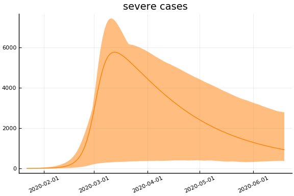
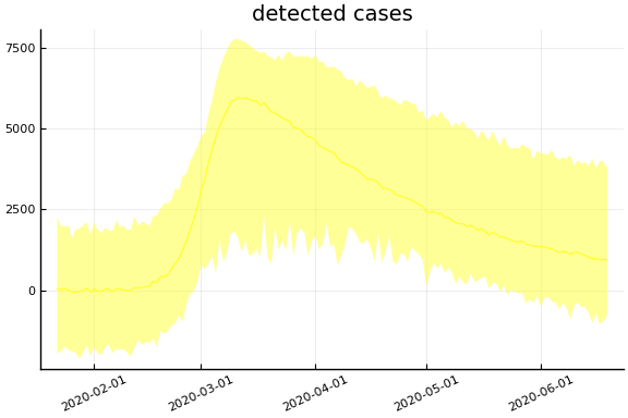
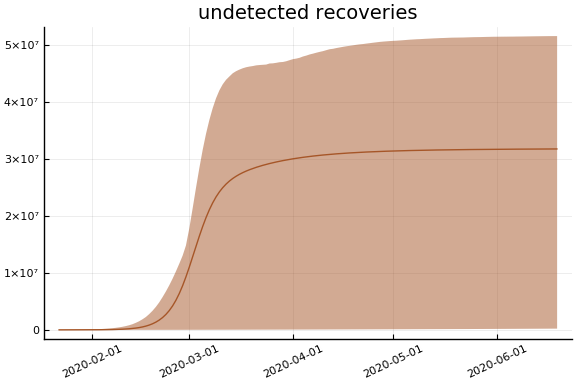
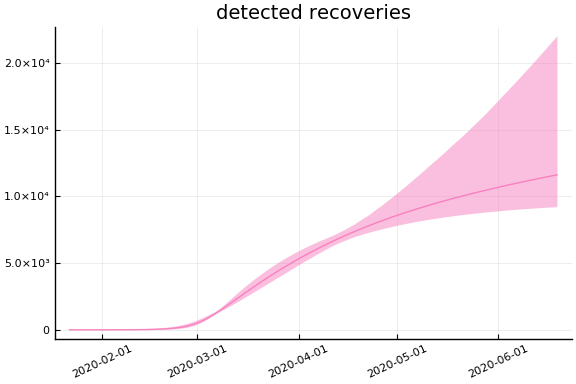
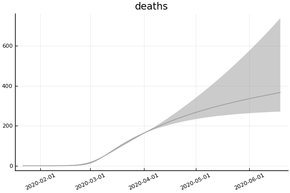
Fit
sdf = simtrajectories(cc, korea, 1:150)
f = plotvars(sdf, korea, dayt0=dayt0)
plot!(f.fit, xlim=nothing)
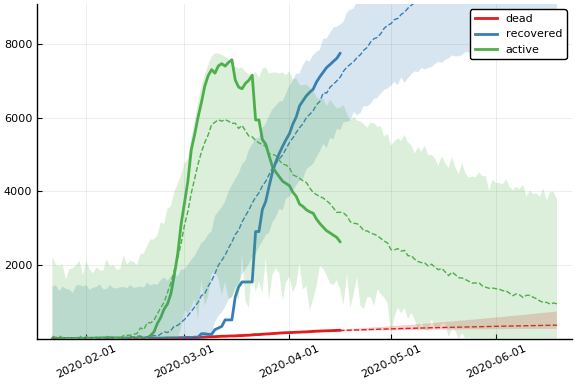
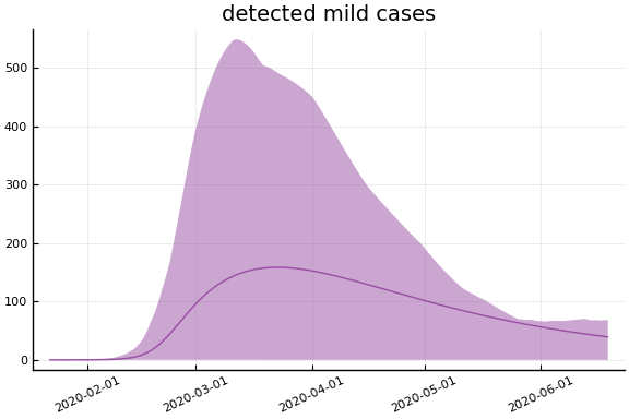
We see that the model does not fit the rapid drop in new cases in South Korea. This may be caused by the model’s implausible assumption that transmission and testing rates are constant over time.
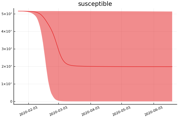
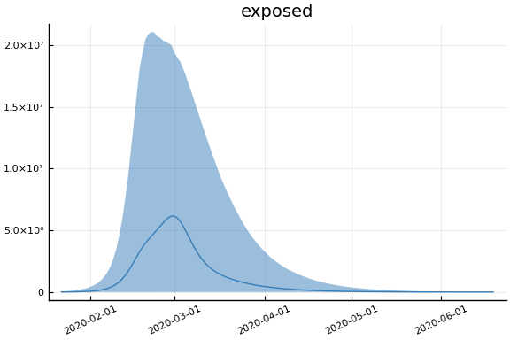
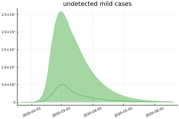
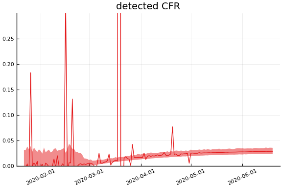
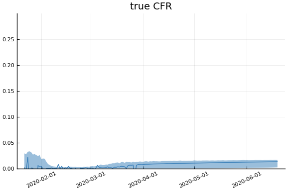
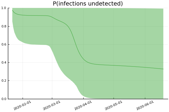
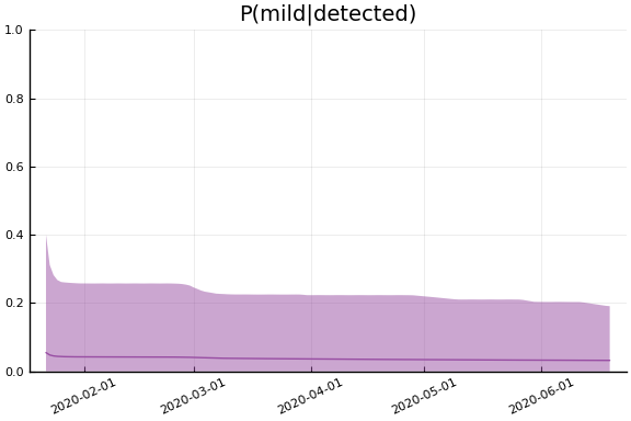
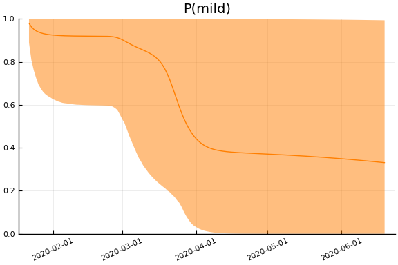
Implications
for fig in f.trajectories
  display(plot(fig, xlim=nothing))
end