This work is licensed under a Creative Commons Attribution-ShareAlike 4.0 International License
using CovidSEIR,  Plots, DataFrames, JLD2, StatsPlots, Dates, MCMCChains
Plots.pyplot()
jmddir = normpath(joinpath(dirname(Base.find_package("CovidSEIR")),"..","docs","jmd"))
covdf = covidjhudata();
United States
us = CountryData(covdf, "US")
CovidSEIR.CountryData{Float64,Int64}(3.2716743e8, [1, 2, 3, 4, 5, 6, 7, 8,
9, 10  …  77, 78, 79, 80, 81, 82, 83, 84, 85, 86], [0.0, 0.0, 0.0, 0.0, 0.0
, 0.0, 0.0, 0.0, 0.0, 0.0  …  12722.0, 14695.0, 16478.0, 18586.0, 20462.0,
22019.0, 23528.0, 25831.0, 28325.0, 32916.0], [0.0, 0.0, 0.0, 0.0, 0.0, 0.0
, 0.0, 0.0, 0.0, 0.0  …  21763.0, 23559.0, 25410.0, 28790.0, 31270.0, 32988
.0, 43482.0, 47763.0, 52096.0, 54703.0], [1.0, 1.0, 2.0, 2.0, 5.0, 5.0, 5.0
, 5.0, 5.0, 7.0  …  361738.0, 390798.0, 419549.0, 449159.0, 474664.0, 50030
6.0, 513609.0, 534076.0, 555929.0, 580182.0])
using Turing
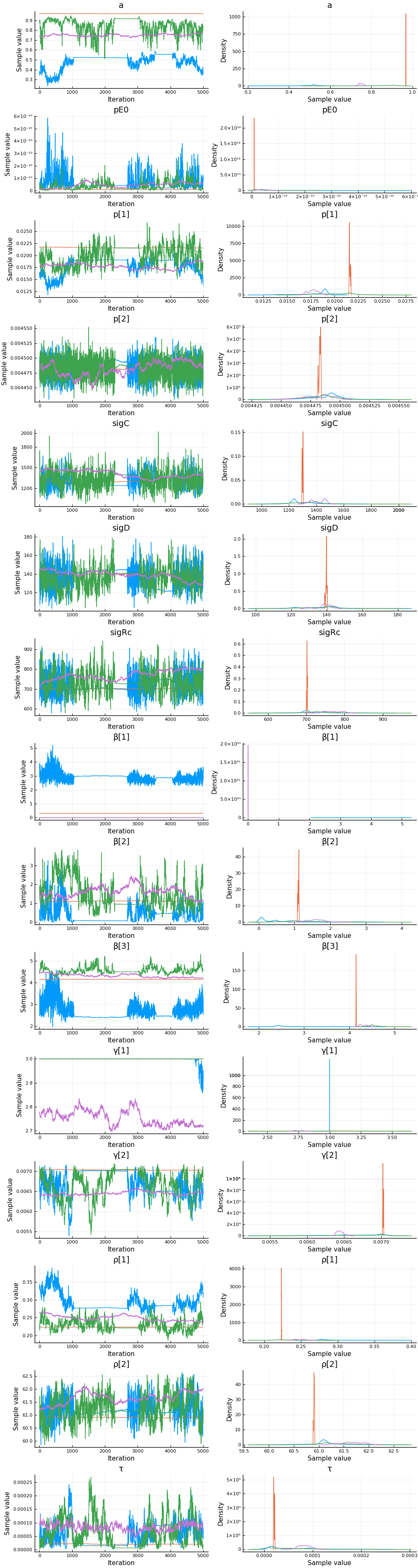
mdl = CovidSEIR.TimeVarying.countrymodel(us)
cc = Turing.psample(mdl, NUTS(0.65), 5000, 4)
import JLD2
JLD2.@save "$jmddir/us_tv_$(Dates.today()).jld2" cc
JLD2.@load "$jmddir/us_dhmc_2020-04-13.jld2" cc;
cc = MCMCChains.Chains(collect(cc.value.data), replace.(cc.name_map.parameters, r"([^\[])([1-9])" => s"\1[\2]"))
Object of type Chains, with data of type 5000×15×4 Array{Float64,3}

Iterations        = 1:5000
Thinning interval = 1
Chains            = 1, 2, 3, 4
Samples per chain = 5000
parameters        = τ, sigD, sigC, sigRc, a, pE0, p[1], p[2], β[1], β[2], β
[3], γ[1], γ[2], ρ[1], ρ[2]

2-element Array{MCMCChains.ChainDataFrame,1}

Summary Statistics
  parameters       mean      std  naive_se    mcse       ess   r_hat
  ──────────  ─────────  ───────  ────────  ──────  ────────  ──────
           τ     0.0001   0.0000    0.0000  0.0000   81.9924  1.2819
        sigD   137.7127   8.0087    0.0566  0.3734  140.4813  1.0810
        sigC  1334.2734  92.6313    0.6550  4.5797   97.6593  1.2625
       sigRc   731.7612  43.2561    0.3059  2.2038   96.7621  1.2997
           a     0.7609   0.1862    0.0013  0.0131   80.3213  3.9037
         pE0     0.0000   0.0000    0.0000  0.0000  100.5049  1.1776
        p[1]     0.0193   0.0021    0.0000  0.0001   80.3213  1.7318
        p[2]     0.0045   0.0000    0.0000  0.0000  141.0271  1.0764
        β[1]     0.8113   1.2418    0.0088  0.0876   80.3213  9.1362
        β[2]     1.1373   0.6511    0.0046  0.0422   80.3213  1.5722
        β[3]     3.9270   0.7566    0.0053  0.0529   80.3213  3.8765
        γ[1]     2.9379   0.1078    0.0008  0.0076   80.3213  7.4234
        γ[2]     0.0067   0.0003    0.0000  0.0000   80.3213  1.4663
        ρ[1]     0.2486   0.0306    0.0002  0.0021   80.3213  2.2939
        ρ[2]    61.2539   0.4053    0.0029  0.0241   80.3213  1.3951

Quantiles
  parameters       2.5%      25.0%      50.0%      75.0%      97.5%
  ──────────  ─────────  ─────────  ─────────  ─────────  ─────────
           τ     0.0000     0.0000     0.0000     0.0001     0.0002
        sigD   118.6077   135.2341   139.7070   141.1686   152.2954
        sigC  1155.0157  1294.3130  1305.6873  1394.1663  1504.5102
       sigRc   653.7688   701.9086   724.4422   762.5418   816.5018
           a     0.3665     0.5791     0.7621     0.9520     0.9683
         pE0     0.0000     0.0000     0.0000     0.0000     0.0000
        p[1]     0.0151     0.0178     0.0190     0.0216     0.0223
        p[2]     0.0045     0.0045     0.0045     0.0045     0.0045
        β[1]     0.0000     0.0000     0.1534     0.7802     3.2127
        β[2]     0.0723     0.7875     1.1188     1.5326     2.6644
        β[3]     2.4007     4.1450     4.1807     4.4108     4.7409
        γ[1]     2.7158     2.8516     3.0000     3.0000     3.0000
        γ[2]     0.0061     0.0064     0.0067     0.0070     0.0070
        ρ[1]     0.2132     0.2236     0.2414     0.2667     0.3312
        ρ[2]    60.5702    60.9084    61.1496    61.5801    62.0245
Estimates
plot(cc)
describe(cc)
2-element Array{MCMCChains.ChainDataFrame,1}

Summary Statistics
  parameters       mean      std  naive_se    mcse       ess   r_hat
  ──────────  ─────────  ───────  ────────  ──────  ────────  ──────
           τ     0.0001   0.0000    0.0000  0.0000   81.9924  1.2819
        sigD   137.7127   8.0087    0.0566  0.3734  140.4813  1.0810
        sigC  1334.2734  92.6313    0.6550  4.5797   97.6593  1.2625
       sigRc   731.7612  43.2561    0.3059  2.2038   96.7621  1.2997
           a     0.7609   0.1862    0.0013  0.0131   80.3213  3.9037
         pE0     0.0000   0.0000    0.0000  0.0000  100.5049  1.1776
        p[1]     0.0193   0.0021    0.0000  0.0001   80.3213  1.7318
        p[2]     0.0045   0.0000    0.0000  0.0000  141.0271  1.0764
        β[1]     0.8113   1.2418    0.0088  0.0876   80.3213  9.1362
        β[2]     1.1373   0.6511    0.0046  0.0422   80.3213  1.5722
        β[3]     3.9270   0.7566    0.0053  0.0529   80.3213  3.8765
        γ[1]     2.9379   0.1078    0.0008  0.0076   80.3213  7.4234
        γ[2]     0.0067   0.0003    0.0000  0.0000   80.3213  1.4663
        ρ[1]     0.2486   0.0306    0.0002  0.0021   80.3213  2.2939
        ρ[2]    61.2539   0.4053    0.0029  0.0241   80.3213  1.3951

Quantiles
  parameters       2.5%      25.0%      50.0%      75.0%      97.5%
  ──────────  ─────────  ─────────  ─────────  ─────────  ─────────
           τ     0.0000     0.0000     0.0000     0.0001     0.0002
        sigD   118.6077   135.2341   139.7070   141.1686   152.2954
        sigC  1155.0157  1294.3130  1305.6873  1394.1663  1504.5102
       sigRc   653.7688   701.9086   724.4422   762.5418   816.5018
           a     0.3665     0.5791     0.7621     0.9520     0.9683
         pE0     0.0000     0.0000     0.0000     0.0000     0.0000
        p[1]     0.0151     0.0178     0.0190     0.0216     0.0223
        p[2]     0.0045     0.0045     0.0045     0.0045     0.0045
        β[1]     0.0000     0.0000     0.1534     0.7802     3.2127
        β[2]     0.0723     0.7875     1.1188     1.5326     2.6644
        β[3]     2.4007     4.1450     4.1807     4.4108     4.7409
        γ[1]     2.7158     2.8516     3.0000     3.0000     3.0000
        γ[2]     0.0061     0.0064     0.0067     0.0070     0.0070
        ρ[1]     0.2132     0.2236     0.2414     0.2667     0.3312
        ρ[2]    60.5702    60.9084    61.1496    61.5801    62.0245
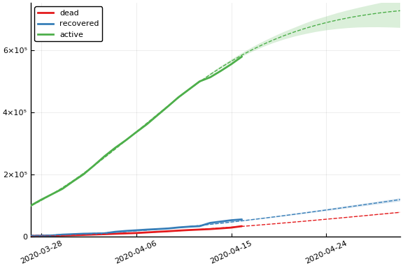
Fit
sdf = simtrajectories(cc, us, 1:200)
f = plotvars(sdf, us)
plot(f.fit, ylim=(0, maximum(us.active)*1.3))
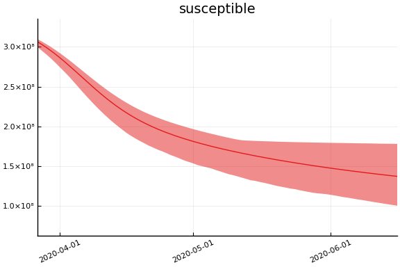
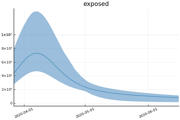
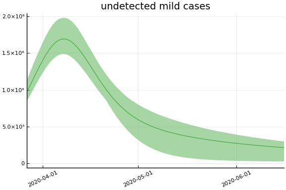
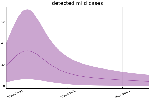
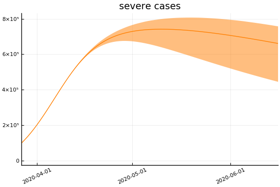
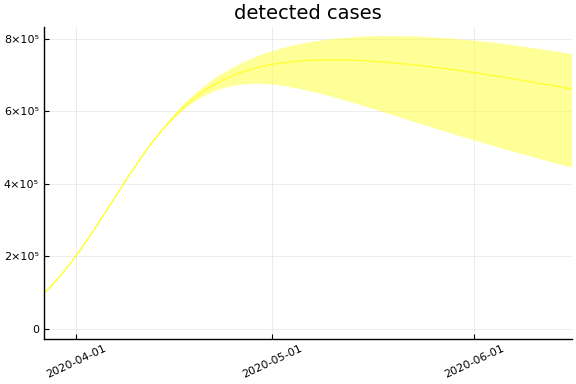
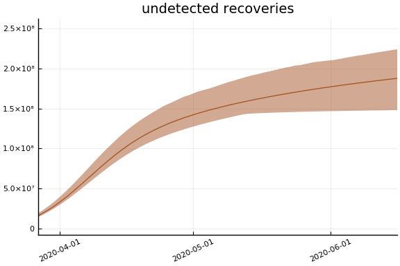
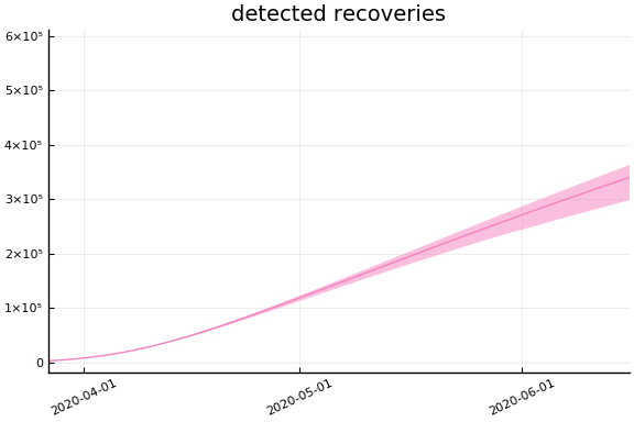
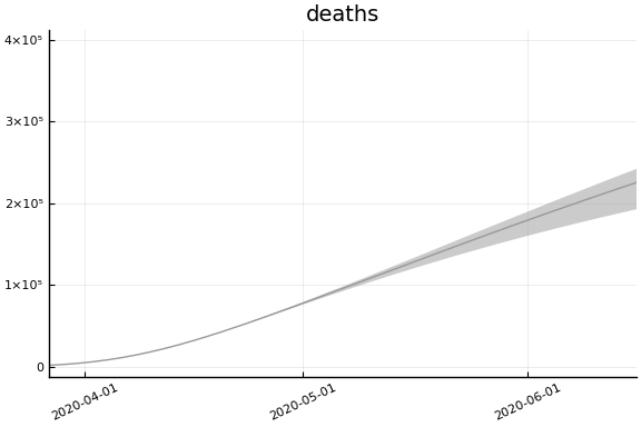
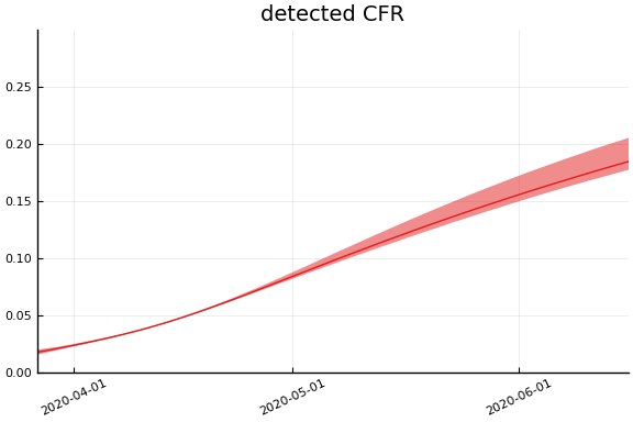
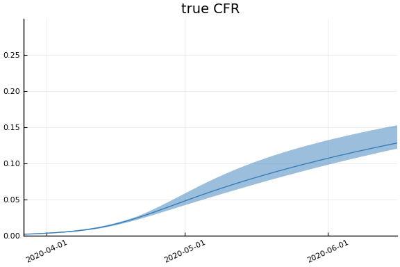
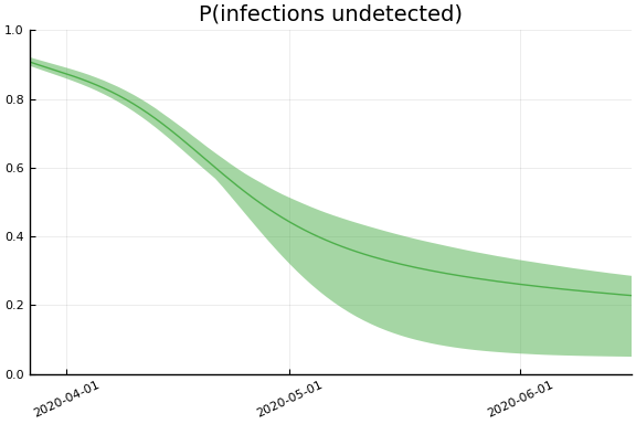
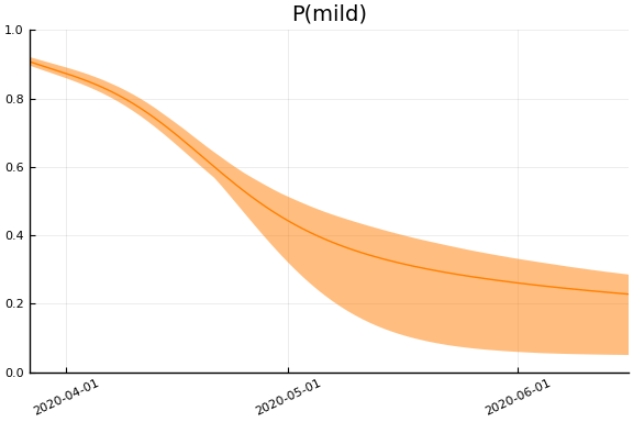
Implications
for fig in f.trajectories
  display(plot(fig))
end