This work is licensed under a Creative Commons Attribution-ShareAlike 4.0 International License
using CovidSEIR,  Plots, DataFrames, JLD2, StatsPlots, MCMCChains
Plots.pyplot()
jmddir = normpath(joinpath(dirname(Base.find_package("CovidSEIR")),"..","docs","jmd"))
covdf = covidjhudata();
China
using Dates
dayt0 = Dates.Date("2020-01-22") - Dates.Day(65)
china = CountryData(covdf, "China", 65)
CovidSEIR.CountryData{Float64,Int64}(1.39273e9, [65, 66, 67, 68, 69, 70, 71
, 72, 73, 74  …  141, 142, 143, 144, 145, 146, 147, 148, 149, 150], [17.0,
18.0, 26.0, 42.0, 56.0, 82.0, 131.0, 133.0, 171.0, 213.0  …  3335.0, 3337.0
, 3339.0, 3340.0, 3343.0, 3343.0, 3345.0, 3345.0, 3346.0, 3346.0], [28.0, 3
0.0, 36.0, 39.0, 49.0, 58.0, 101.0, 120.0, 135.0, 214.0  …  77410.0, 77567.
0, 77679.0, 77791.0, 77877.0, 77956.0, 78039.0, 78200.0, 78311.0, 78401.0],
 [503.0, 595.0, 858.0, 1325.0, 1970.0, 2737.0, 5277.0, 5834.0, 7835.0, 9375
.0  …  1973.0, 1905.0, 1865.0, 1810.0, 1794.0, 1835.0, 1829.0, 1761.0, 1699
.0, 1656.0])
using Turing
mdl = CovidSEIR.TimeVarying.countrymodel(china)
cc = Turing.psample(mdl, NUTS(0.65), 5000, 4)
import JLD2
JLD2.@save "$jmddir/china_$(Dates.today()).jld2" cc dayt0
JLD2.@load "$jmddir/china_dhmc_2020-04-13.jld2" cc dayt0;
cc = MCMCChains.Chains(collect(cc.value.data), replace.(cc.name_map.parameters, r"([^\[])([1-9])" => s"\1[\2]"))
Object of type Chains, with data of type 5000×15×4 Array{Float64,3}

Iterations        = 1:5000
Thinning interval = 1
Chains            = 1, 2, 3, 4
Samples per chain = 5000
parameters        = τ, sigD, sigC, sigRc, a, pE0, p[1], p[2], β[1], β[2], β
[3], γ[1], γ[2], ρ[1], ρ[2]

2-element Array{MCMCChains.ChainDataFrame,1}

Summary Statistics
  parameters        mean        std  naive_se      mcse       ess    r_hat
  ──────────  ──────────  ─────────  ────────  ────────  ────────  ───────
           τ      0.0000     0.0000    0.0000    0.0000   80.3213   1.5862
        sigD     90.1865   108.1679    0.7649    7.6652   80.3213  16.4095
        sigC  12749.7844  4659.6012   32.9484  322.0747   80.3213   4.5433
       sigRc   8238.5858  3466.7500   24.5136  242.3239   80.3213   4.9360
           a      0.7721     0.1378    0.0010    0.0069  120.2959   1.1108
         pE0      0.0000     0.0000    0.0000    0.0000   80.3213   1.6474
        p[1]      0.0004     0.0005    0.0000    0.0000   80.3213   7.1795
        p[2]      0.4376     0.4398    0.0031    0.0309   80.3213   6.8857
        β[1]      0.3384     0.3067    0.0022    0.0213   80.3213   2.0684
        β[2]      0.7464     0.6525    0.0046    0.0298  124.5414   1.1639
        β[3]      1.4304     1.4707    0.0104    0.1042   80.3213   9.1300
        γ[1]      1.2668     1.2386    0.0088    0.0878   80.3213  13.3651
        γ[2]      0.1599     0.1464    0.0010    0.0081   86.9155   1.3707
        ρ[1]      0.8703     0.1652    0.0012    0.0117   80.3213   2.2865
        ρ[2]     87.7994     1.4004    0.0099    0.0850   80.3213   1.5699

Quantiles
  parameters       2.5%       25.0%       50.0%       75.0%       97.5%
  ──────────  ─────────  ──────────  ──────────  ──────────  ──────────
           τ     0.0000      0.0000      0.0000      0.0000      0.0000
        sigD    23.6088     26.6456     28.8155     91.4797    292.9900
        sigC  4388.5359  10075.1023  14738.3582  15853.7267  17853.3371
       sigRc  4613.6964   5290.9410   6950.5976  10492.7804  14948.0661
           a     0.4875      0.6742      0.7763      0.8873      0.9793
         pE0     0.0000      0.0000      0.0000      0.0000      0.0000
        p[1]     0.0000      0.0000      0.0001      0.0007      0.0014
        p[2]     0.0021      0.0033      0.1933      0.8908      0.9903
        β[1]     0.0269      0.1482      0.2338      0.3377      1.1417
        β[2]     0.0000      0.2806      0.5279      1.1032      2.3880
        β[3]     0.0530      0.1431      0.8618      2.9038      3.8533
        γ[1]     0.0819      0.0852      0.6694      2.5336      3.0000
        γ[2]     0.0336      0.0461      0.0849      0.2376      0.5292
        ρ[1]     0.4234      0.7741      0.9711      0.9943      0.9995
        ρ[2]    85.6977     86.6899     87.6515     88.7356     90.8120
Estimates
plot(cc)
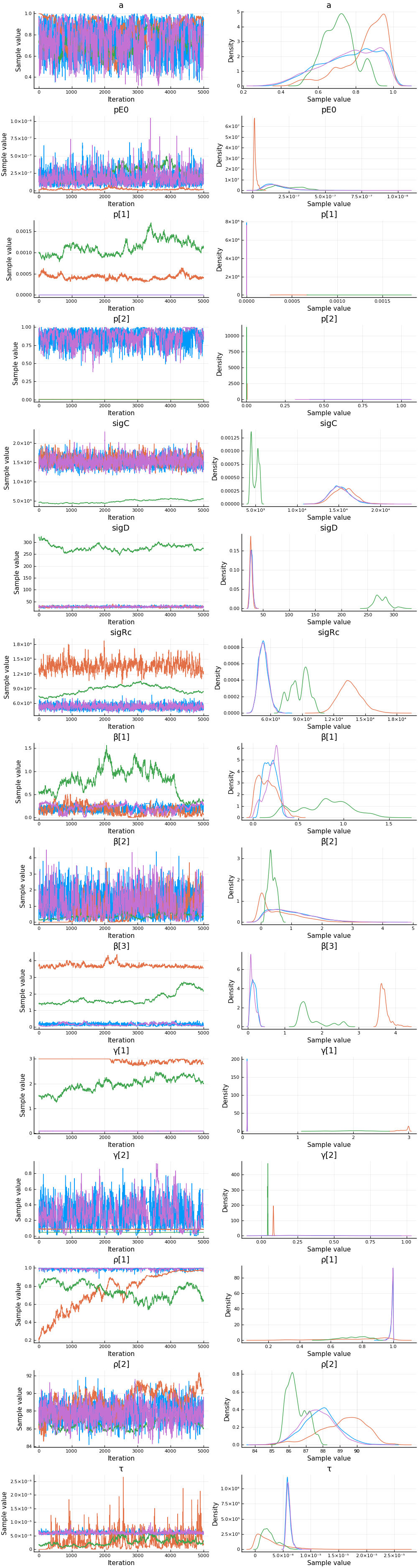
describe(cc)
2-element Array{MCMCChains.ChainDataFrame,1}

Summary Statistics
  parameters        mean        std  naive_se      mcse       ess    r_hat
  ──────────  ──────────  ─────────  ────────  ────────  ────────  ───────
           τ      0.0000     0.0000    0.0000    0.0000   80.3213   1.5862
        sigD     90.1865   108.1679    0.7649    7.6652   80.3213  16.4095
        sigC  12749.7844  4659.6012   32.9484  322.0747   80.3213   4.5433
       sigRc   8238.5858  3466.7500   24.5136  242.3239   80.3213   4.9360
           a      0.7721     0.1378    0.0010    0.0069  120.2959   1.1108
         pE0      0.0000     0.0000    0.0000    0.0000   80.3213   1.6474
        p[1]      0.0004     0.0005    0.0000    0.0000   80.3213   7.1795
        p[2]      0.4376     0.4398    0.0031    0.0309   80.3213   6.8857
        β[1]      0.3384     0.3067    0.0022    0.0213   80.3213   2.0684
        β[2]      0.7464     0.6525    0.0046    0.0298  124.5414   1.1639
        β[3]      1.4304     1.4707    0.0104    0.1042   80.3213   9.1300
        γ[1]      1.2668     1.2386    0.0088    0.0878   80.3213  13.3651
        γ[2]      0.1599     0.1464    0.0010    0.0081   86.9155   1.3707
        ρ[1]      0.8703     0.1652    0.0012    0.0117   80.3213   2.2865
        ρ[2]     87.7994     1.4004    0.0099    0.0850   80.3213   1.5699

Quantiles
  parameters       2.5%       25.0%       50.0%       75.0%       97.5%
  ──────────  ─────────  ──────────  ──────────  ──────────  ──────────
           τ     0.0000      0.0000      0.0000      0.0000      0.0000
        sigD    23.6088     26.6456     28.8155     91.4797    292.9900
        sigC  4388.5359  10075.1023  14738.3582  15853.7267  17853.3371
       sigRc  4613.6964   5290.9410   6950.5976  10492.7804  14948.0661
           a     0.4875      0.6742      0.7763      0.8873      0.9793
         pE0     0.0000      0.0000      0.0000      0.0000      0.0000
        p[1]     0.0000      0.0000      0.0001      0.0007      0.0014
        p[2]     0.0021      0.0033      0.1933      0.8908      0.9903
        β[1]     0.0269      0.1482      0.2338      0.3377      1.1417
        β[2]     0.0000      0.2806      0.5279      1.1032      2.3880
        β[3]     0.0530      0.1431      0.8618      2.9038      3.8533
        γ[1]     0.0819      0.0852      0.6694      2.5336      3.0000
        γ[2]     0.0336      0.0461      0.0849      0.2376      0.5292
        ρ[1]     0.4234      0.7741      0.9711      0.9943      0.9995
        ρ[2]    85.6977     86.6899     87.6515     88.7356     90.8120
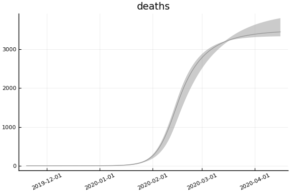
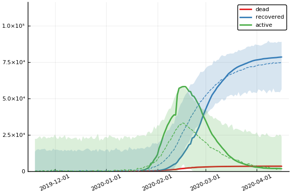
Fit
sdf = simtrajectories(cc, china, 1:150)
f = plotvars(sdf, china, dayt0=dayt0)
plot(f.fit, xlim=nothing, ylim=(0, maximum(china.active)*2))
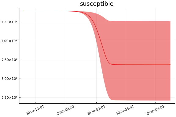
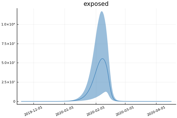
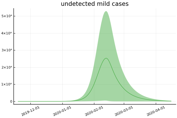
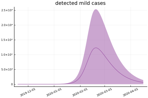
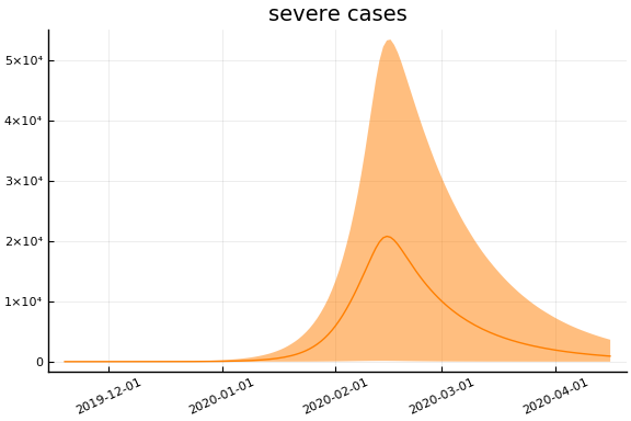
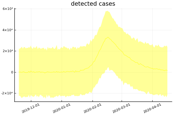
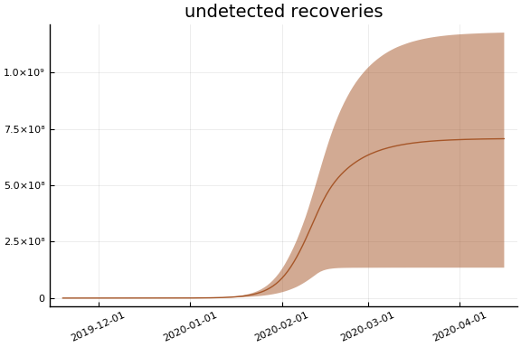
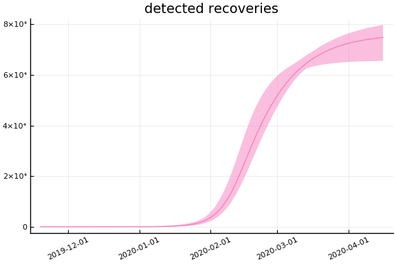
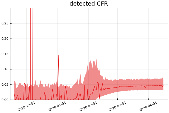
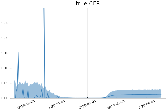
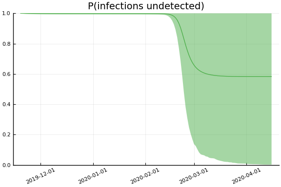
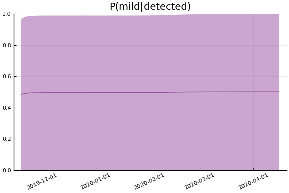
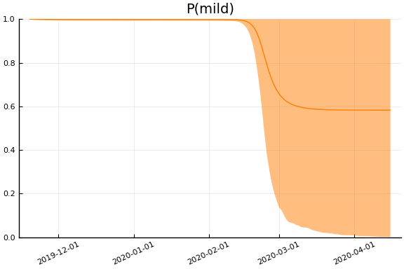
Implications
for fig in f.trajectories
  display(plot(fig, xlim=nothing))
end