Longer Differences and Smoothing¶

One way to reduce $\sigma_k/\sigma_R$ is to reduce noise in new cases by taking a longer difference or smoothing case counts in some other way. How does this affect the estimation and interpretation of $R_t$?

As in the first section, we start with the approximate recursive relation $C(t) - C(t-1) \equiv \Delta C(t) \approx \frac{\tau(t)}{\tau(t-1)} e^{\gamma (R_t - 1)} \Delta C(t-1)$ If we instead look at a longer difference, $\begin{align*} C(t) - C(t-L) = & \sum_{i=0}^{L-1} \Delta C_{t-i} \\ \approx & \sum_{i=0}^{L-1} \frac{\tau(t-i)}{\tau(t-i-1)} e^{\gamma (R_{t-i} - 1)} \Delta C_{t-i-1} \\ = & \overline {T_{t,L} e^{\gamma(R_{t,L} - 1)}} \sum_{i=0}^{L-1}\Delta C_{t-i-1} \\ = & \overline {T_{t,L} e^{\gamma(R_{t,L} - 1)}} \left( C(t-1) - C(t-1-L) \right) \end{align*}$ where $\overline {T_{t,L} e^{\gamma(R_{t,L} - 1)}}$ is some intermediate value in between the minimum and maximum of the ${ \frac{\tau(t-i)}{\tau(t-i-1)} e^{\gamma (R_{t-i} - 1)} }_{i=0}^{L-1}$.

If testing is constant over time, we can then obtain an interpretable $\overline{R_{t,L}}$ by using $k_{t,L} =\log(C(t)-C(t-L))$ and following the procedure above.

If testing varies with time, it becomes hard to separate testing rate changes from $R_t$ after taking long differnces.

Note

The same analysis can be applied to other smoothing operations, i.e. using $\sum_{i=0}^L w_i \Delta C_{t-i}$ in place of $C(t) - C(t-L)$. However, there’s something strange about smoothing $C_t$, and then extracting a smoothed component of it using the Kalman filter. The inference afterwards is suspect; we would essentially be estimating a kernel regression of $C_t$ on time, and using the estimated regression as though it’s known with certainty.

When would long differences reduce variance? Well if $\Delta C(t) = \Delta C^\ast(t) + \epsilon_t$ with $\epsilon_t$ indepenedent over time with mean $0$ and constant variance, then you would need $C^\ast(t) - C^\ast(t-L)$ to increase faster than linearly with $L$. This is true if $C^\ast$ is growing exponentially.

Alternatively, if $\epsilon_t$ is not independent over time, but negatively correlated (as seems likely), then variance can decrease with $L$. For example, if $\Delta C(t) = C^\ast(t) - C^\ast(t-\delta)$ with $\delta$ a random, independent increment with mean $1$, then variance will tend to decrease with $L$ regardless of $C^\ast(t)$.

Results¶

Here, we will allow the initial and time varying mean of $R_{s,t}$ to depend on covariates.

$\begin{align*} \tilde{R}_{s,0} & \sim N(X_{0,s} \alpha_0, \sigma^2_{R,0}) \\ \tilde{R}_{s,t} & = \rho \tilde{R}_{s,t} + u_{s,t} \;,\; u_{s,t} \sim N(0, \sigma^2_R) \\ R_{s,t} & = X_{s,t} \alpha + \tilde{R}_{s,t} \\ \Delta \log(k)_{s,t} & = \gamma (R_{s,t} - 1) + \epsilon_{s,t} - \epsilon_{s,t-1} \;, \; \epsilon_{s,t} \sim N(0, \sigma^2_k) \end{align*}$

reestimate=false
rlo=-1 #1 - eps(Float64)
rhi=1.2 #1+ eps(Float64)
K = size(X[1],2)
priors = (γ = truncated(Normal(1/7,1/7), 1/28, 1/1),
          σR0 = truncated(Normal(1, 3), 0, Inf),
          α0 = MvNormal(zeros(length(X0[1])), sqrt(10)), #truncated(Normal(1, 3), 0, Inf),
          σR = truncated(Normal(0.25,1),0,Inf),
          σk = truncated(Normal(0.1, 5), 0, Inf),
          ρ = Uniform(rlo, rhi),
          α = MvNormal(zeros(K), sqrt(10))
          )
mdl = RT.RtRW(dlogk, X, X0, priors);
trans = as( (γ = asℝ₊, σR0 = asℝ₊, α0 = as(Array, length(X0[1])),
             σR = asℝ₊, σk = asℝ₊, ρ=as(Real, rlo, rhi),
             α = as(Array, K)) )
P = TransformedLogDensity(trans, mdl)
∇P = ADgradient(:ForwardDiff, P)

p0 = (γ = 1/7, σR0=1.0, α0 = zeros(length(X0[1])), σR=0.25, σk=2.0, ρ=1.0, α=zeros(K))
x0 = inverse(trans,p0)
@time LogDensityProblems.logdensity_and_gradient(∇P, x0);

2.090468 seconds (4.01 M allocations: 193.476 MiB, 9.03% gc time)

rng = MersenneTwister()
steps = 100
warmup=default_warmup_stages(local_optimization=nothing, #FindLocalOptimum(1e-6, 200),
                             stepsize_search=nothing,
                             init_steps=steps, middle_steps=steps,
                             terminating_steps=2*steps,  doubling_stages=4, M=Symmetric)
x0 = x0
if !isfile("rt7.jld2") || reestimate
   res = DynamicHMC.mcmc_keep_warmup(rng, ∇P, 2000;initialization = (q = x0, ϵ=0.1),
                                      reporter = LogProgressReport(nothing, 25, 15),
                                                                 warmup_stages =warmup);
   post = transform.(trans,res.inference.chain)
   @save "rt7.jld2" post
end
@load "rt7.jld2" post
p = post[1]
vals = hcat([vcat([length(v)==1 ? v : vec(v) for v in values(p)]...) for p in post]...)'
vals = reshape(vals, size(vals)..., 1)
names = vcat([length(p[s])==1 ? String(s) : String.(s).*"[".*string.(1:length(p[s])).*"]" for s in keys(p)]...)
cc = MCMCChains.Chains(vals, names)
display(plot(cc))

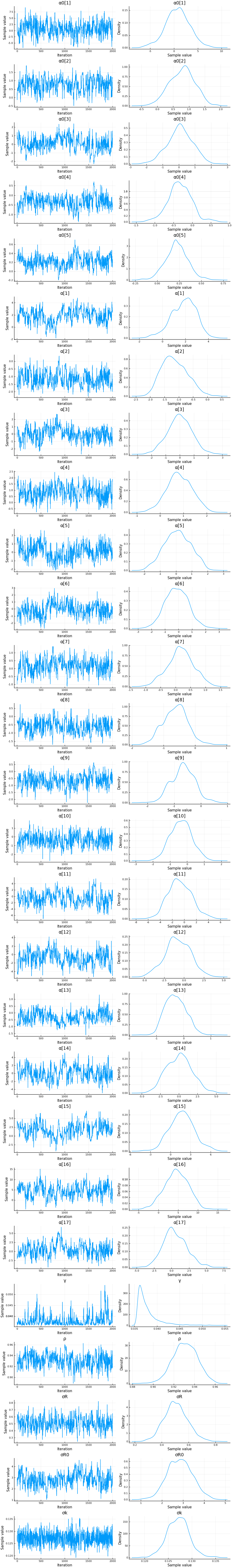
display(describe(cc))

2-element Array{ChainDataFrame,1}

Summary Statistics
  parameters     mean     std  naive_se    mcse       ess   r_hat
  ──────────  ───────  ──────  ────────  ──────  ────────  ──────
           γ   0.0379  0.0025    0.0001  0.0003  108.5762  1.0094
         σR0   2.8472  0.5901    0.0132  0.0656   48.7521  1.0343
       α0[1]   0.7643  2.5342    0.0567  0.1661  187.4434  1.0018
       α0[2]   0.7817  0.3966    0.0089  0.0296  171.7902  1.0026
       α0[3]   0.0789  0.7772    0.0174  0.0986   37.6326  1.0154
       α0[4]  -0.3337  0.3151    0.0070  0.0315   82.1813  1.0035
       α0[5]   0.2207  0.1280    0.0029  0.0147   47.5974  1.0322
          σR   0.5057  0.0870    0.0019  0.0041  255.7555  1.0007
          σk   0.1271  0.0024    0.0001  0.0001  446.0680  0.9998
           ρ   0.9309  0.0116    0.0003  0.0010  107.4759  1.0163
        α[1]   1.8516  1.0681    0.0239  0.1446   25.1433  1.0501
        α[2]  -1.1438  0.4449    0.0099  0.0416  105.1060  1.0127
        α[3]  -0.0083  0.8520    0.0191  0.1048   44.8124  1.0340
        α[4]   0.8243  0.5430    0.0121  0.0493  124.4263  1.0032
        α[5]   0.0994  0.8315    0.0186  0.1093   31.5759  0.9995
        α[6]  -0.1280  0.8602    0.0192  0.1103   40.2397  0.9995
        α[7]   0.1713  0.4355    0.0097  0.0390  160.8671  1.0006
        α[8]  -0.6264  0.3775    0.0084  0.0300  124.0985  1.0104
        α[9]  -0.6664  0.4365    0.0098  0.0395   96.5867  1.0059
       α[10]  -0.3495  0.6313    0.0141  0.0483  173.2760  0.9999
       α[11]  -0.7192  1.9604    0.0438  0.2069   78.9574  1.0042
       α[12]  -0.7804  1.5990    0.0358  0.1891   39.9999  1.0244
       α[13]  -0.2912  0.3787    0.0085  0.0497   38.9951  1.0060
       α[14]   0.0375  1.7094    0.0382  0.2016   77.1582  1.0000
       α[15]   1.6999  1.8242    0.0408  0.2300   52.0837  1.0387
       α[16]   4.5390  2.9292    0.0655  0.3112   78.9740  1.0021
       α[17]   0.5028  1.6706    0.0374  0.2142   47.3735  1.0128

Quantiles
  parameters     2.5%    25.0%    50.0%    75.0%    97.5%
  ──────────  ───────  ───────  ───────  ───────  ───────
           γ   0.0358   0.0363   0.0370   0.0385   0.0447
         σR0   1.7240   2.4285   2.8403   3.2445   4.0325
       α0[1]  -4.6969  -0.8651   0.8286   2.4189   5.8212
       α0[2]   0.0048   0.5012   0.8055   1.0475   1.5065
       α0[3]  -1.4842  -0.4245   0.0886   0.6008   1.5086
       α0[4]  -0.9854  -0.5299  -0.3391  -0.1320   0.3514
       α0[5]  -0.0282   0.1411   0.2189   0.2999   0.4784
          σR   0.3405   0.4481   0.5033   0.5608   0.6871
          σk   0.1224   0.1255   0.1272   0.1286   0.1318
           ρ   0.9081   0.9232   0.9311   0.9394   0.9532
        α[1]  -0.4662   1.1087   1.9482   2.6229   3.7126
        α[2]  -1.8904  -1.4731  -1.1892  -0.8362  -0.2449
        α[3]  -1.6674  -0.5660  -0.0063   0.5603   1.6550
        α[4]  -0.2679   0.4651   0.8096   1.2006   1.8807
        α[5]  -1.5504  -0.4773   0.1007   0.7080   1.6550
        α[6]  -1.7526  -0.7365  -0.1388   0.4751   1.5934
        α[7]  -0.6846  -0.1063   0.1747   0.4540   1.0258
        α[8]  -1.3522  -0.8877  -0.6086  -0.3772   0.1172
        α[9]  -1.4709  -0.9545  -0.6563  -0.3671   0.2092
       α[10]  -1.5648  -0.7817  -0.3454   0.0693   0.8933
       α[11]  -4.1944  -2.0611  -0.8113   0.6417   3.3614
       α[12]  -4.0476  -1.7987  -0.7897   0.3959   2.3293
       α[13]  -0.9347  -0.5773  -0.3129  -0.0225   0.4680
       α[14]  -3.1091  -1.2218   0.0735   1.1604   3.4156
       α[15]  -1.7118   0.4843   1.7194   2.8932   5.6024
       α[16]  -1.3076   2.5101   4.5436   6.6371   9.8855
       α[17]  -2.5148  -0.6405   0.3466   1.6276   3.9682

display([1:length(x0vars)  x0vars])

5×2 Array{Any,2}:
 1  :constant
 2  :logpopdens
 3  Symbol("Percent.Unemployed..2018.")
 4  Symbol("Percent.living.under.the.federal.poverty.line..2018.")
 5  Symbol("Percent.at.risk.for.serious.illness.due.to.COVID")

display([1:length(xvars) xvars])

17×2 Array{Any,2}:
  1  :constant
  2  Symbol("Stay.at.home..shelter.in.place")
  3  Symbol("State.of.emergency")
  4  Symbol("Date.closed.K.12.schools")
  5  Symbol("Closed.gyms")
  6  Symbol("Closed.movie.theaters")
  7  Symbol("Closed.day.cares")
  8  Symbol("Date.banned.visitors.to.nursing.homes")
  9  Symbol("Closed.non.essential.businesses")
 10  Symbol("Closed.restaurants.except.take.out")
 11  :retail_and_recreation_percent_change_from_baseline
 12  :grocery_and_pharmacy_percent_change_from_baseline
 13  :parks_percent_change_from_baseline
 14  :transit_stations_percent_change_from_baseline
 15  :workplaces_percent_change_from_baseline
 16  :residential_percent_change_from_baseline
 17  :percentchangebusinesses

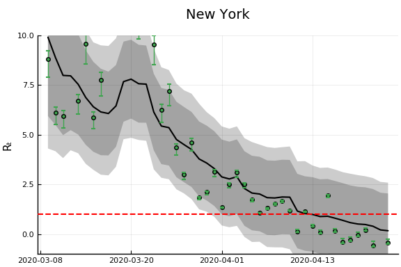
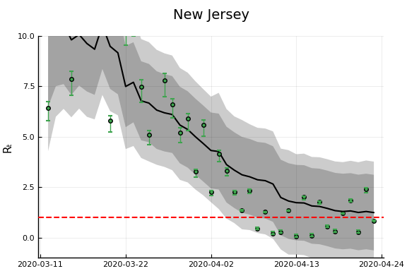
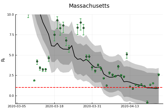
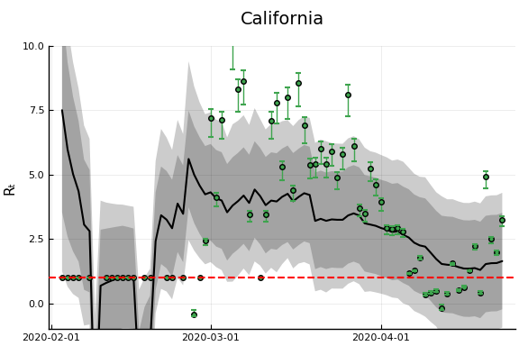
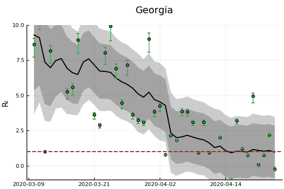
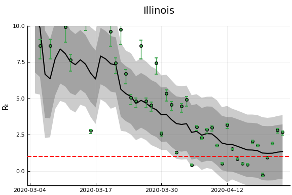
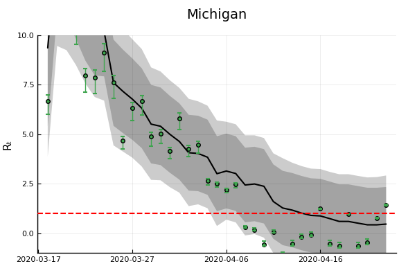
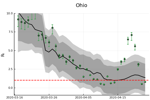
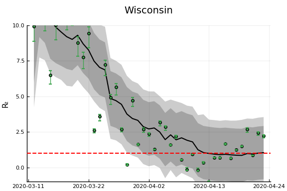
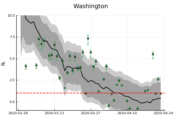
states = unique(sdf.state)
states_to_plot = ["New York", "New Jersey","Massachusetts","California",
                  "Georgia","Illinois","Michigan",
                  "Ohio","Wisconsin","Washington"]
S = length(states_to_plot)
figs = fill(plot(), S)
for (i,st) in enumerate(states_to_plot)
  s = findfirst(states.==st)
  figr = RT.plotpostr(dates[s],dlogk[s],post, X[s], X0[s])
  l = @layout [a{.1h}; grid(1,1)]
  figs[i] = plot(plot(annotation=(0.5,0.5, st), framestyle = :none),
                 plot(figr, ylim=(-1,10)), layout=l)
  display(figs[i])
end

Another Derivation¶

An alternative (and easier) way to derive the same estimator will be described here. This approach will easily generalize to more complicated models, but let’s begin with the simplest SIR model with testing.

$\begin{align*} \dot{S} & = -\frac{S}{N} \beta I \\ \dot{I} & = \frac{S}{N} \beta I - \gamma I \\ \dot{C} & = \tau I \\ \dot{\mathcal{R}} & = \gamma I \end{align*}$

Then note that

$\ddot{C} = \dot{\tau} I + \tau \dot{I}$

and

$\begin{align*} \frac{\ddot{C}}{\dot{C}} = & \frac{\dot{\tau}}{\tau} + \frac{\dot{I}}{I} \\ \frac{d}{dt} \log(\dot{C}) = & \frac{\dot{\tau}}{\tau} + \frac{S}{N}\beta - \gamma \\ = & \frac{\dot{\tau}}{\tau} + \gamma(R_t - 1) \end{align*}$

which is the equation we have been using for estimation.

Incorporating death¶

If we add deaths to the model, $\begin{align*} \dot{S} & = -\frac{S}{N} \beta I \\ \dot{I} & = \frac{S}{N} \beta I - \gamma I - p I\\ \dot{C} & = \tau I \\ \dot{\mathcal{R}} & = \gamma I \\ \dot{D} & = p I \end{align*}$

then,

$\begin{align*} \frac{\ddot{C}}{\dot{C}} = & \frac{\dot{\tau}}{\tau} + \frac{S}{N}\beta - \gamma - p \\ \frac{\ddot{D}}{\dot{D}} = & \frac{S}{N}\beta - \gamma - p \\ \end{align*}$

Other observable states could similarly be added to the model.

Time delays¶

A drawback of the above approach is that it implies changes in $R_t$ show up in the derivatives of case and death numbers instantly. This is definitely not true. Instead consider a model where infections last $\ell$ days. After $\ell$ days, each infected person dies with probability $\pi$ and recovers otherwise. Then we have

$\begin{align*} \dot{S}(t) & = -\frac{S(t)}{N} \beta I \\ \dot{I}(t) & = \frac{S(t)}{N} \beta(t) I(t) - \frac{S(t-\ell)}{N} \beta(t-\ell) I(t-\ell) \\ \dot{C}(t) & = \tau(t) I(t) \\ \dot{\mathcal{R}}(t) & = (1-\pi) \frac{S(t-\ell)}{N} \beta(t-\ell) I(t-\ell) \\ \dot{D}(t) & = \pi \frac{S(t-\ell)}{N} \beta(t-\ell) I(t-\ell) \end{align*}$

Rearranging gives $\frac{\ddot{C}(t)}{\dot{C}(t)} = \frac{\dot{\tau}(t)}{\tau(t)} + \frac{S(t)}{N}\beta(t) - \frac{1}{\pi} \frac{\dot{D}(t)}{\dot{C}(t)}$ and $\dot{D}(t) = \pi \frac{S(t-\ell)}{N} \beta(t-\ell) \frac{\dot{C}(t-\ell)}{\tau(t-\ell)}$

Note

These last two equations also hold in the model without time delay by setting $\ell=0$ and $\pi = \frac{p}{p+\gamma}$

Note

Random durations can be accomodated by replacing the shift by $\ell$ with a convolution.

Keys	Action
`?`	Open this help
`n`	Next page
`p`	Previous page
`s`	Search